Elevation Model Conditioning and Stream Network Delimitation with Python and Pysheds - Tutorial
/Never before the process of watershed delimitation became so easy. Now you can delimitate your watershed and stream network online with Hatari Utils:
Check this tutorial:
hatarilabs.com/ih-en/online-watershed-delimitation-with-hatari-utils-tutorial
In modern history, computer algorithms can interpret hydrological features from a topographical relief. Following the definition of a drainage basin, all water that precipitates on an area should drain in a common outlet with gravity as the only driving force. For a “hydrological correct” basin topography, all the drainage network should have a downward path to the discharge point, therefore any sink or depression would “stop” the surface runoff pathway and the computer won’t intrepret the river network.
Digital elevation models (DEMs) from satellite interpretation (Aster DEM or Alos Palsar) come with “sinks” from errors in the elevation interpretation, raster resolution or reprojection. There is a need to correct those rasters in order to interpret the hydrological features. This tutorial show the process to condition a digital elevation model (DEM) dowloaded from a NASA/USGS server (gdex.cr.usgs.gov) with the Pysheds library of Python. The tutorial was done on a Jupyter Notebook, input files and scripts are attached on the final part of the post.
Pysheds
There are new features in Pysheds for basin and stream network delimitation. To the date of this post (22-01-2019) the latest version of Pysheds allows the use of digital elevation models in both geograpical coordinates (WGS84) and projected coordinates (WGS 84 UTM). This feature increase the versatility of the hydrological analysis.
The two Pysheds set of commands used for this tutorial for DEM conditioning were:
Detect and fill depressions
Detect and resolve flats
Usually depressions are not easy to identify on a visual inspection because they are located in a small number of cells. Once Pysheds have filled the depressions, it has to resolve the flat parts on the modified DEM.
Elevation representation with stream network
Depressions on the DEM (red pixels)
Flat parts after the depression fill
Final and corrected topography on the stream network is different from the original as it can be seen on the following figure. The original surface topography is on dark blue, while the corrected elevation is shown in light blue.
Cross section along a part the river network (yellow line). Done with QGIS 3 and Profile Tool plugin.
Tutorial
Python code
This is the python code for this tutorial:
#Import required libraries
import numpy as np
import matplotlib.pyplot as plt
import matplotlib.colors as colors
import geopandas as gpd
from pysheds.grid import Grid
import mplleaflet
%matplotlib inline
#Open a digital elevation model
grid = Grid.from_raster('../Rst/20190109125130_1063922483.tif', data_name='dem')#Define a function to plot the digital elevation model
def plotFigure(data, label, cmap='Blues'):
plt.figure(figsize=(12,10))
plt.imshow(data, extent=grid.extent)
plt.colorbar(label=label)
plt.grid()#Minnor slicing on borders to enhance colobars
elevDem=grid.dem[:-1,:-1]plotFigure(elevDem, 'Elevation (m)')# Detect depressions
# Detect depressions
depressions = grid.detect_depressions('dem')
# Plot depressions
plt.imshow(depressions)# Fill depressions
grid.fill_depressions(data='dem', out_name='flooded_dem')# Test result
depressions = grid.detect_depressions('flooded_dem')
plt.imshow(depressions)# Detect flats
flats = grid.detect_flats('flooded_dem')
# Plot flats
plt.imshow(flats)grid.resolve_flats(data='flooded_dem', out_name='inflated_dem')
plt.imshow(grid.inflated_dem[:-1,:-1])# Create a flow direction grid
#N NE E SE S SW W NW
dirmap = (64, 128, 1, 2, 4, 8, 16, 32)grid.flowdir(data='inflated_dem', out_name='dir', dirmap=dirmap)plotFigure(grid.dir,'Flow Direction','viridis')# Specify discharge point
x, y = -107.91663,27.83479# Delineate the catchment
grid.catchment(data='dir', x=x, y=y, dirmap=dirmap, out_name='catch',
recursionlimit=15000, xytype='label', nodata_out=0)# Clip the bounding box to the catchment
grid.clip_to('catch')# Get a view of the catchment
demView = grid.view('dem', nodata=np.nan)plotFigure(demView,'Elevation')#export selected raster
grid.to_raster(demView, '../Output/clippedElevations_WGS84.tif')# Define the stream network
grid.accumulation(data='catch', dirmap=dirmap, pad_inplace=False, out_name='acc')
accView = grid.view('acc', nodata=np.nan)
plotFigure(accView,"Cell Number",'PuRd')streams = grid.extract_river_network('catch', 'acc', threshold=200, dirmap=dirmap)
streams["features"][:2]def saveDict(dic,file):
f = open(file,'w')
f.write(str(dic))
f.close()#save geojson as separate file
saveDict(streams,'../Output/streams_WGS84.geojson')# Some functions to plot the json on jupyter notebook
streamNet = gpd.read_file('../Output/streams_WGS84.geojson')
streamNet.crs = {'init' :'epsg:4326'}# The polygonize argument defaults to the grid mask when no arguments are supplied
shapes = grid.polygonize()
# Plot catchment boundaries
fig, ax = plt.subplots(figsize=(6.5, 6.5))
for shape in shapes:
coords = np.asarray(shape[0]['coordinates'][0])
ax.plot(coords[:,0], coords[:,1], color='cyan')
ax.set_xlim(grid.bbox[0], grid.bbox[2])
ax.set_ylim(grid.bbox[1], grid.bbox[3])
ax.set_title('Catchment boundary (vector)')
gpd.plotting.plot_dataframe(streamNet, None, cmap='Blues', ax=ax)#ax = streamNet.plot()
mplleaflet.display(fig=ax.figure, crs=streamNet.crs, tiles='esri_aerial')Input data
You can download the input data for this tutorial here.


