How to create a MODFLOW 6 model from geospatial data with Python and Flopy - Tutorial
/Nature is geospatial, and every physical process related to the groundwater flow and transport regime is spatially located or spatially distributed. Groundwater models are based on a grid structure and models are discretized on cells located on arrangements of rows and columns; is that level of disconnexion of the spatial position of a piece of porous media and the corresponding cell, row and column that creates some challenges for the sustainable management of groundwater resources.
We have developed an applied case of groundwater model discretized from ESRI Shapefiles with refinement areas. Boundary conditions are also set up from spatial data with the intersect functionality of Flopy. Model surface and layer bottom are imported / processed from xyz point data. The simulation is run for one steady and ten transient stress periods and results are plotted for head on aerial view and cross section.
Tutorial
Code
This is the main Python code for model creation.
Import the required libraries
#!pip install pyshp
#!pip install geopandas
#!pip install folium
import numpy as np
import matplotlib.pyplot as plt
import flopy
import geopandas as gpd
import pandas as pd
import folium
from scipy.interpolate import griddata
from shapely.geometry import MultiLineString
from workingFunctions import *
Refinement areas and spatial / temporal discretization
# Open the shapefiles from the model limit and the refiment area around the wells
modelLimitShp = gpd.read_file('../Shp/ModelLimit1.shp')
modelWelShp = gpd.read_file('../Shp/ModelWell2.shp')
fig, ax = plt.subplots()
modelLimitShp.plot(ax=ax, facecolor='none', ec='royalblue')
modelWelShp.plot(ax=ax, color='crimson')
plt.show()#Since we have geospatial and georeferenced data, we can add a satellite image in the background with Folium
modelLimitWgs = modelLimitShp.to_crs('4326')
modelWelWgs = modelWelShp.to_crs('4326')
center = modelLimitWgs.geometry.centroid.iloc[0].coords[0][::-1]
center
# Initialize a Folium map centered on the data
m = folium.Map(location=center, zoom_start=15)
# Add GeoDataFrame as GeoJSON to the map
folium.GeoJson(modelLimitWgs).add_to(m)
folium.GeoJson(modelWelWgs).add_to(m)
# Display the map
mC:\Users\GIDA\AppData\Local\Temp\ipykernel_6048\1142086283.py:5: UserWarning: Geometry is in a geographic CRS. Results from 'centroid' are likely incorrect. Use 'GeoSeries.to_crs()' to re-project geometries to a projected CRS before this operation.
center = modelLimitWgs.geometry.centroid.iloc[0].coords[0][::-1]# Coordinates of the global and local discretization
GloRefBox = modelLimitShp.total_bounds
LocRefBox = modelWelShp.total_bounds
print(GloRefBox)
print(LocRefBox)[ 353300. 8547900. 356400. 8549600.]
[ 354369.88403372 8548609.34745342 354904.62742419 8549128.04875159]#Calculating Global Model (Glo) and Local Refinement (Loc) dimensions
GloLx = GloRefBox[2] - GloRefBox[0] #x_max - x_min
GloLy = GloRefBox[3] - GloRefBox[1]
print('Global Refinement Dimension. Easting Dimension: %8.1f, Northing Dimension: %8.1f' % (GloLx,GloLy))
LocLx = LocRefBox[2] - LocRefBox[0] #x_max - x_min
LocLy = LocRefBox[3] - LocRefBox[1]
print('Local Refinement Dimension. Easting Dimension: %8.1f, Northing Dimension: %8.1f' % (LocLx,LocLy))Global Refinement Dimension. Easting Dimension: 3100.0, Northing Dimension: 1700.0
Local Refinement Dimension. Easting Dimension: 534.7, Northing Dimension: 518.7#Defining Global and Local Refinements, for purpose of simplicity cell x and y dimension will be the same
celGlo = 100
celRef = 50#Remember that DELR is space between rows, so it is the column dimension array
delRArray = arrayGeneratorCol(GloRefBox, LocRefBox, celGlo, celRef)
delRArrayarray([100., 100., 100., 100., 100., 100., 100., 100., 100., 100., 50.,
50., 50., 50., 50., 50., 50., 50., 50., 50., 50., 50.,
50., 50., 50., 100., 100., 100., 100., 100., 100., 100., 100.,
100., 100., 100., 100., 100., 100.])#And DELC is the space between columns, so its the row dimension array
delCArray = arrayGeneratorRow(GloRefBox, LocRefBox, celGlo, celRef)
delCArrayarray([100., 100., 100., 100., 50., 50., 50., 50., 50., 50., 50.,
50., 50., 50., 50., 50., 50., 50., 100., 100., 100., 100.,
100., 100.])#Calculating number or rows and cols since they are dependant from the discretization
nrows = delCArray.shape[0]
ncols = delRArray.shape[0]
print('Number of rows: %d and number of cols: %d' % (nrows,ncols))Number of rows: 24 and number of cols: 39Creation of model object and application of MODFLOW NWT
simName = 'Sim1'

modelWs = '../Model'
exeName = '../Exe/mf6.exe'

sim = flopy.mf6.MFSimulation(sim_name=simName, exe_name=exeName, version='mf6', sim_ws=modelWs)
# Create the solver (IMS) package
ims = flopy.mf6.ModflowIms(sim, print_option="SUMMARY", complexity="SIMPLE")# Create the time discretization package
nper = 11
perlen = np.ones(nper)
perlen[0] = 1
perlen[1:] = 200 * 86400
nstp = np.ones(nper)
nstp[1:] = 4
perioddata = []
for per,stp in zip(perlen,nstp):
perioddata.append((per, stp, 1.0))
print(perioddata[:5])
tdis = flopy.mf6.ModflowTdis(sim, time_units='SECONDS', nper=nper, perioddata=perioddata)[(1.0, 1.0, 1.0), (17280000.0, 4.0, 1.0), (17280000.0, 4.0, 1.0), (17280000.0, 4.0, 1.0), (17280000.0, 4.0, 1.0)]# Create the groundwater flow (GWF) model
modelName = 'Model1'
gwf = flopy.mf6.ModflowGwf(sim, modelname=modelName, save_flows=True)#Definition of stress period type, transient or steady state
periodType = np.zeros(11, dtype=bool)
periodType[0] = True#Number of layers and temporal layer elevations
nlays = 3
mtop = 0
botm = [-10,-20,-30]
# Apply the spatial parameters to the DIS package
dis = flopy.mf6.ModflowGwfdis(gwf,
xorigin=GloRefBox[0], yorigin=GloRefBox[1],
angrot=0,
nlay=nlays, nrow=nrows, ncol=ncols,
delr=delRArray, delc=delCArray,
top=mtop, botm=botm,
)#Assign spatial reference
#Actually, this only works for metadata
gwf.modelgrid.crs = '32718'
gwf.modelgrid.origin = (GloRefBox[0], GloRefBox[3])
gwf.modelgrid.rotation = 0.0fig = plt.figure(figsize=(8,8))
ax = fig.add_subplot(1, 1, 1, aspect='equal')
modelmap = flopy.plot.PlotMapView(model=gwf)
linecollection = modelmap.plot_grid(linewidth=0.5, color='royalblue')#Representation of model geometry with all the boundary conditions
fig, ax = plt.subplots()
modelmap = flopy.plot.PlotMapView(model=gwf)
linecollection = modelmap.plot_grid(linewidth=0.5, color='cyan', ax=ax)
shpRiver = flopy.plot.plot_shapefile('../Shp/ModelRiver2', ax=ax) #RIV boundary condition
shpGHB = flopy.plot.plot_shapefile('../Shp/ModelGHB1', ax=ax) #GHB boundary condition
modelWelShp.plot(ax=ax)<Axes: >Definition of Model Top and Layer Bottom Elevation for the UPW package
dem = pd.read_csv('../Rst/ModeloDem2.csv')
dem.head()| Easting | Northing | Elevation | |
|---|---|---|---|
| 0 | 353214.799 | 8549716.14 | 58.925 |
| 1 | 353245.085 | 8549716.14 | 59.267 |
| 2 | 353275.372 | 8549716.14 | 59.609 |
| 3 | 353305.658 | 8549716.14 | 59.951 |
| 4 | 353335.945 | 8549716.14 | 60.293 |
points = dem[['Easting','Northing']].values
values = dem['Elevation'].values
grid_x = gwf.modelgrid.xcellcenters
grid_y = gwf.modelgrid.ycellcenters
mtop = griddata(points, values, (grid_x, grid_y), method='nearest')
mtop[:5,:5]
array([[60.293, 61.661, 62.686, 63.712, 65.08 ],
[60.293, 61.661, 62.686, 63.712, 65.08 ],
[60.293, 61.661, 62.686, 63.712, 65.08 ],
[60.293, 61.661, 62.686, 63.712, 65.08 ],
[60.293, 61.661, 62.686, 63.712, 65.08 ]])fig, ax = plt.subplots()
modelmap = flopy.plot.PlotMapView(model=gwf,ax=ax)
ax.set_aspect('equal')
quadmesh = modelmap.plot_array(mtop)#Asign surface elevations
gwf.dis.top = mtop
AcuifInf_Bottom = -120
AcuifMed_Bottom = AcuifInf_Bottom + (0.5 * (mtop - AcuifInf_Bottom))
AcuifSup_Bottom = AcuifInf_Bottom + (0.75 * (mtop - AcuifInf_Bottom))
zbot = np.zeros((nlays,nrows,ncols))
zbot[0,:,:] = AcuifSup_Bottom
zbot[1,:,:] = AcuifMed_Bottom
zbot[2,:,:] = AcuifInf_Bottom
#Asign layer bottom elevations
gwf.dis.botm = zbotfig, ax = plt.subplots()
modelxsect = flopy.plot.PlotCrossSection(model=gwf, line={'Row': 20})
linecollection = modelxsect.plot_grid()Kx = np.zeros((nlays,nrows,ncols))
Kx[0,:,:] = 1E-5 #first layer of lime
Kx[1,:,:] = 5E-4 #second layer of sand
Kx[2,:,:] = 2E-4 #third layer of sandy gravelfig, ax = plt.subplots()
modelxsect = flopy.plot.PlotCrossSection(model=gwf, line={'Row': 20})
linecollection = modelxsect.plot_grid()
modelxsect.plot_array(Kx)
print(Kx[:,10,10]) #print values of K for all layers in cell row / col = 10 , 10[1.e-05 5.e-04 2.e-04]# Initial conditions package
ic = flopy.mf6.ModflowGwfic(gwf, strt=100.0)
# Definition of layer type, the first two layers are convertible
icelltype = [1,1,0]
# Node property flow package (hydraulic conductivity)
npf = flopy.mf6.ModflowGwfnpf(gwf, icelltype=icelltype, k=Kx)# Add storage package
transient = [False] + [True for i in range(nper-1)]
sto = flopy.mf6.ModflowGwfsto(gwf, transient = transient)Definition of the intersect object
For the manipulation of spatial data to determine hydraulic parameters or boundary conditions
# Define intersection object
interIx = flopy.utils.gridintersect.GridIntersect(gwf.modelgrid)
Recharge and Evapotranspiration as RCH and EVT boundary condition
# We apply recharge to the extension of the irrigated areas and evapotranspiration to the whole extent,
# The recharge rate is estimated in 200 mm /yr and the potential evapotraspiration is 1200 mm/yr

# Evapotranspiration rate
evtr = 1.2 / 365. / 86400. # 1200 mm/yr in m/s
evt = flopy.mf6.ModflowGwfevta(gwf, surface=mtop, rate=evtr, depth=1.0)
# Open the recharge polygon
rechDf = gpd.read_file('../Shp/ModelRechargeZone1.shp')
rechPoly = rechDf.iloc[0].geometry
rechPolyrechResult = interIx.intersect(rechPoly)
rechResult.cellids[:5]array([(0, 0), (0, 1), (0, 2), (0, 3), (0, 4)], dtype=object)rechRate = 0.2 / 365. / 86400.
rech_spd = {} # empty dictionary for all stress periods, actually spd comes from stress period data
rech_spd[0] = np.zeros([nrows,ncols])
for cell in rechResult.cellids:
rech_spd[0][cell] = rechRate
rch = flopy.mf6.ModflowGwfrcha(gwf,recharge=rech_spd)rch.plot(mflay=0)[<Axes: title={'center': 'RECHARGE stress period 1'}>]Recharge and Evapotranspiration as RCH and EVT boundary condition
modelWelShp.iloc[0].geometry
wel1 = interIx.intersect(modelWelShp.iloc[0].geometry).cellids
wel2 = interIx.intersect(modelWelShp.iloc[1].geometry).cellids
wel3 = interIx.intersect(modelWelShp.iloc[2].geometry).cellids
wel3
array([(5, 15)], dtype=object)welSpd = {}
welSpd[0] = []
welSpd[1] = [((1,wel1[0][0],wel1[0][1]),-0.03),
((1,wel2[0][0],wel2[0][1]),-0.03),
((1,wel3[0][0],wel3[0][1]),-0.03)]
wel = flopy.mf6.ModflowGwfwel(gwf, stress_period_data=welSpd)wel.plot(kper=1, mflay=1)[<Axes: title={'center': ' wel_0 location stress period 2 layer 2'}>]River path as RIV boundary condition
riverDf = gpd.read_file('../Shp/ModelRiver2.shp')
riverDf.iloc[0].geometry
riverIx = interIx.intersect(riverDf.iloc[0].geometry).cellids
riverIx[:5]array([(6, 25), (6, 26), (6, 32), (6, 33), (6, 34)], dtype=object)riverSpd = {}
riverSpd[0] = []
for cell in riverIx:
i, j = cell
riverSpd[0].append([(0,i,j),mtop[i,j],0.01,mtop[i,j]-1])
riv = flopy.mf6.ModflowGwfriv(gwf, stress_period_data=riverSpd)riv.plot(mflay=0)[<Axes: title={'center': ' riv_0 location stress period 1 layer 1'}>]Regional flow as GHB boundary condition
ghbDf = gpd.read_file('../Shp/ModelGHB1.shp')
ghbLines = MultiLineString([line for line in ghbDf.geometry])
ghbLines
ghbIx = interIx.intersect(ghbLines).cellids
ghbIx[:5]array([(0, 0), (1, 0), (2, 0), (3, 0), (4, 0)], dtype=object)ghbSpd = {}
ghbSpd[0] = []
for cell in ghbIx:
i, j = cell
if j == 0:
ghbSpd[0].append([(0,i,j),55,0.01])
elif j == ncols-1:
ghbSpd[0].append([(0,i,j),90,0.01])
else:
print('Wrong')
ghb = flopy.mf6.ModflowGwfghb(gwf, stress_period_data=ghbSpd)ghb.plot(mflay=0)[<Axes: title={'center': ' ghb_0 location stress period 1 layer 1'}>]Set the Output Control and run simulation
#oc = flopy.modflow.ModflowOc(mf, stress_period_data=oc_spd)
head_filerecord = f"{gwf.name}.hds"
oc = flopy.mf6.ModflowGwfoc(gwf,
                            head_filerecord=head_filerecord,
                            saverecord=[("HEAD", "LAST")])
# Run the simulation
sim.write_simulation()
success, buff = sim.run_simulation()writing simulation...
writing simulation name file...
writing simulation tdis package...
writing solution package ims_-1...
writing model Model1...
writing model name file...
writing package dis...
writing package ic...
writing package npf...
writing package sto...
writing package evta_0...
writing package rcha_0...
writing package wel_0...
INFORMATION: maxbound in ('gwf6', 'wel', 'dimensions') changed to 3 based on size of stress_period_data
writing package riv_0...
INFORMATION: maxbound in ('gwf6', 'riv', 'dimensions') changed to 93 based on size of stress_period_data
writing package ghb_0...
INFORMATION: maxbound in ('gwf6', 'ghb', 'dimensions') changed to 36 based on size of stress_period_data
writing package oc...
FloPy is using the following executable to run the model: ..\Exe\mf6.exe
MODFLOW 6
U.S. GEOLOGICAL SURVEY MODULAR HYDROLOGIC MODEL
VERSION 6.5.0 05/23/2024
MODFLOW 6 compiled May 23 2024 18:06:57 with Intel(R) Fortran Intel(R) 64
Compiler Classic for applications running on Intel(R) 64, Version 2021.7.0
Build 20220726_000000
This software has been approved for release by the U.S. Geological
Survey (USGS). Although the software has been subjected to rigorous
review, the USGS reserves the right to update the software as needed
pursuant to further analysis and review. No warranty, expressed or
implied, is made by the USGS or the U.S. Government as to the
functionality of the software and related material nor shall the
fact of release constitute any such warranty. Furthermore, the
software is released on condition that neither the USGS nor the U.S.
Government shall be held liable for any damages resulting from its
authorized or unauthorized use. Also refer to the USGS Water
Resources Software User Rights Notice for complete use, copyright,
and distribution information.
MODFLOW runs in SEQUENTIAL mode
Run start date and time (yyyy/mm/dd hh:mm:ss): 2024/11/08 10:21:40
Writing simulation list file: mfsim.lst
Using Simulation name file: mfsim.nam
Solving: Stress period: 1 Time step: 1
Solving: Stress period: 2 Time step: 1
Solving: Stress period: 2 Time step: 2
Solving: Stress period: 2 Time step: 3
Solving: Stress period: 2 Time step: 4
Solving: Stress period: 3 Time step: 1
Solving: Stress period: 3 Time step: 2
Solving: Stress period: 3 Time step: 3
Solving: Stress period: 3 Time step: 4
Solving: Stress period: 4 Time step: 1
Solving: Stress period: 4 Time step: 2
Solving: Stress period: 4 Time step: 3
Solving: Stress period: 4 Time step: 4
Solving: Stress period: 5 Time step: 1
Solving: Stress period: 5 Time step: 2
Solving: Stress period: 5 Time step: 3
Solving: Stress period: 5 Time step: 4
Solving: Stress period: 6 Time step: 1
Solving: Stress period: 6 Time step: 2
Solving: Stress period: 6 Time step: 3
Solving: Stress period: 6 Time step: 4
Solving: Stress period: 7 Time step: 1
Solving: Stress period: 7 Time step: 2
Solving: Stress period: 7 Time step: 3
Solving: Stress period: 7 Time step: 4
Solving: Stress period: 8 Time step: 1
Solving: Stress period: 8 Time step: 2
Solving: Stress period: 8 Time step: 3
Solving: Stress period: 8 Time step: 4
Solving: Stress period: 9 Time step: 1
Solving: Stress period: 9 Time step: 2
Solving: Stress period: 9 Time step: 3
Solving: Stress period: 9 Time step: 4
Solving: Stress period: 10 Time step: 1
Solving: Stress period: 10 Time step: 2
Solving: Stress period: 10 Time step: 3
Solving: Stress period: 10 Time step: 4
Solving: Stress period: 11 Time step: 1
Solving: Stress period: 11 Time step: 2
Solving: Stress period: 11 Time step: 3
Solving: Stress period: 11 Time step: 4
Run end date and time (yyyy/mm/dd hh:mm:ss): 2024/11/08 10:21:41
Elapsed run time: 0.272 Seconds
Normal termination of simulation.Model output visualization
headObj = gwf.output.head()
headObj.get_kstpkper()
[(0, 0),
(3, 1),
(3, 2),
(3, 3),
(3, 4),
(3, 5),
(3, 6),
(3, 7),
(3, 8),
(3, 9),
(3, 10)]headEnd = headObj.get_data((3,10))
headEnd[0,:5,:5]array([[57.26145566, 62.08668325, 63.04324044, 63.69447381, 64.38216177],
[57.25551222, 62.06935318, 63.02540058, 63.67804767, 64.36583795],
[57.24233563, 62.03378122, 62.9896688 , 63.64520708, 64.33307364],
[57.19230668, 61.97369448, 62.93592401, 63.59605941, 64.28355383],
[56.34462852, 61.87233109, 62.88161668, 63.54712051, 64.23318429]])# Plot the heads for a defined layer and boundary conditions
fig = plt.figure()
ax = fig.add_subplot(1, 1, 1, aspect='equal')
modelmap = flopy.plot.PlotMapView(model=gwf)
contour = modelmap.contour_array(headEnd[1],ax=ax)
quadmesh = modelmap.plot_bc('RIV')
cellhead = modelmap.plot_array(headEnd[1],ax=ax, cmap='Blues', alpha=0.2)
ax.clabel(contour)
plt.tight_layout()
# Boundary conditions
shpGHB = flopy.plot.plot_shapefile('../Shp/ModelGHB1', ax=ax,linewidth=8)
shpWel = flopy.plot.plot_shapefile('../Shp/ModelWell2', ax=ax,radius=20)
shpRiv = flopy.plot.plot_shapefile('../Shp/ModelRiver2', ax=ax)
linecollection = modelmap.plot_grid(linewidth=0.5, alpha=0.5,color='cyan', ax=ax)fig = plt.figure(figsize=(20, 3))
ax = fig.add_subplot(1, 1, 1)
modelxsect = flopy.plot.PlotCrossSection(model=gwf, line={'Row': 10})
linecollection = modelxsect.plot_grid()
modelxsect.contour_array(headEnd)<matplotlib.tri._tricontour.TriContourSet at 0x192b245ee10>


