How to reach small discretizations efficiently (till 1m) in MODFLOW6 with mf6Voronoi - Tutorial
/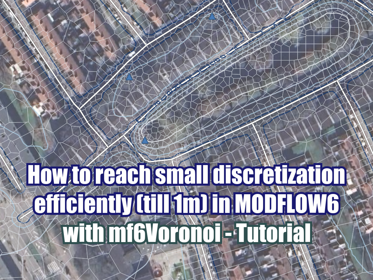
One of the promises of the Voronoi meshes on MODFLOW6 Disv is the efficient distribution of cell sizes that allows us to reach small sizes on certain areas of high interest like wells while keeping coarse cells on the areas with lower level of interest. This type of meshing has some issues that now are addressed on mf6Voronoi.
For example, if we want to create a mesh for a place in Netherlands where the cell sizes go from 50m to 1m we can end up with a mesh distribution like this.
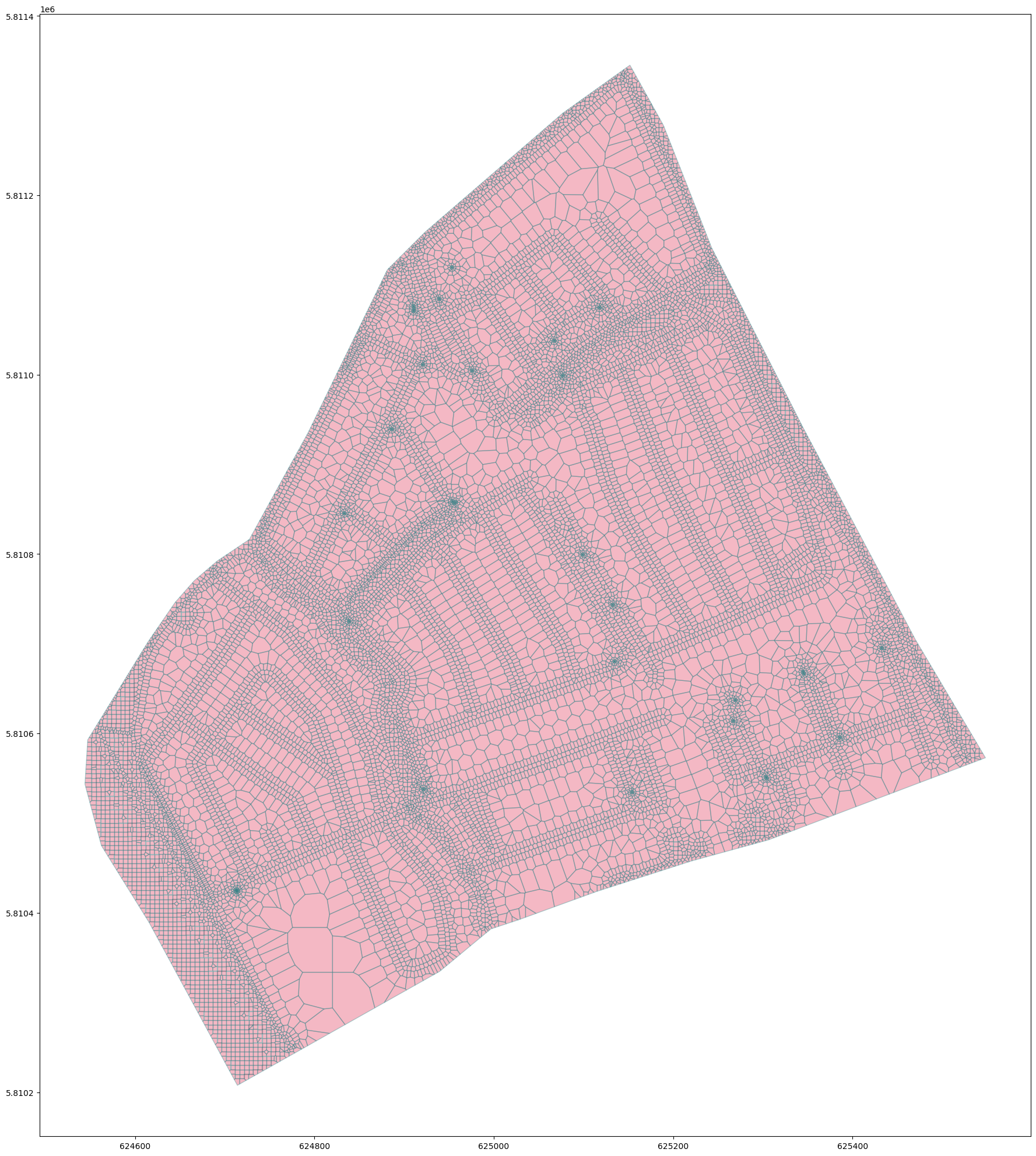
Voronoi discretization over the model limit
We can check that the cell sizes reaches the desired discretization.
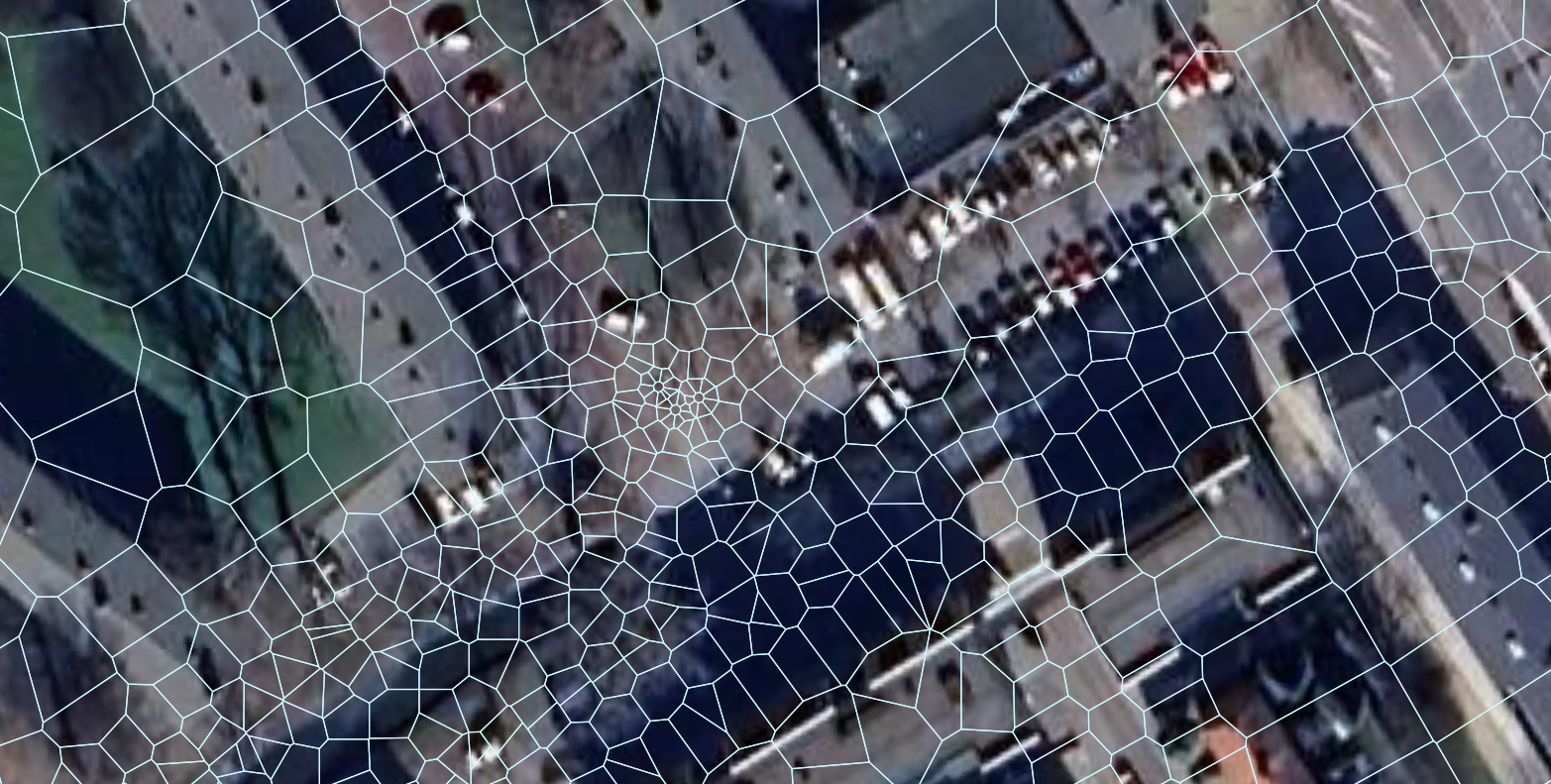
Refinement of 1m around wells and 5m around drains
But we face a problem when we run the model.
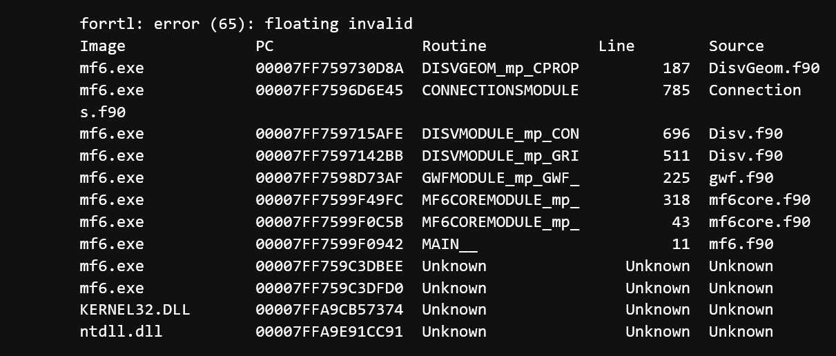
FORTRAN ERROR RELATED TO ISSUES ON THE DISCRETIZATION
But there are tools in mf6Voronoi to adress the short edges on the mesh.
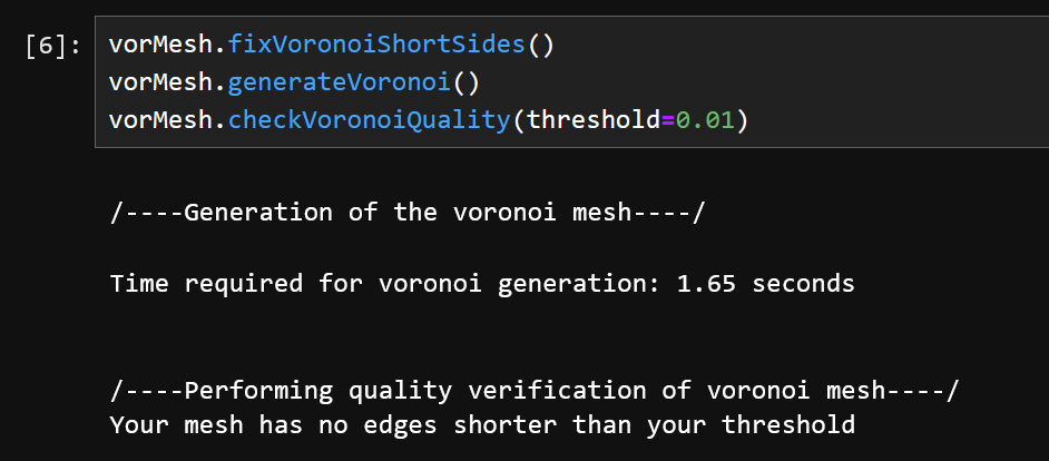
TOOLS on mf6voronoi to fix short sides
Tutorial
Code
For voronoi generation
Part 1 : Voronoi mesh generation
import warnings ## Org
warnings.filterwarnings('ignore') ## Org

import os, sys ## Org
import geopandas as gpd ## Org
from mf6Voronoi.geoVoronoi import createVoronoi ## Org
from mf6Voronoi.meshProperties import meshShape ## Org
from mf6Voronoi.utils import initiateOutputFolder, getVoronoiAsShp ## Org
#Create mesh object specifying the coarse mesh and the multiplier
vorMesh = createVoronoi(meshName='zaandam',maxRef = 50, multiplier=1.8) ## Org
#Open limit layers and refinement definition layers
vorMesh.addLimit('limit','../shp/modelLimit.shp') ## Org
vorMesh.addLayer('wells','../shp/modelWell.shp',1) ## Org
vorMesh.addLayer('drain','../shp/modelDrain.shp',5) ## Org
vorMesh.addLayer('channels','../shp/modelGhb.shp',5) ## Org#Generate point pair array
vorMesh.generateOrgDistVertices() ## Org
#Generate the point cloud and voronoi
vorMesh.createPointCloud() ## Org
vorMesh.generateVoronoi() ## Org
build faster, analyze more
Follow us: |
 |
 |
 |
 |
 |
 |
/--------Layer wells discretization-------/
Progressive cell size list: [1, 2.8, 6.04, 11.872, 22.3696, 41.265280000000004] m.

/--------Layer drain discretization-------/
Progressive cell size list: [5, 14.0, 30.200000000000003] m.

/--------Layer channels discretization-------/
Progressive cell size list: [5, 14.0, 30.200000000000003] m.

/----Sumary of points for voronoi meshing----/
Distributed points from layers: 3
Points from layer buffers: 11274
Points from max refinement areas: 24
Points from min refinement areas: 2397
Total points inside the limit: 16203
/--------------------------------------------/

Time required for point generation: 2.75 seconds


/----Generation of the voronoi mesh----/

Time required for voronoi generation: 1.90 seconds
#Uncomment the next two cells if you have strong differences on discretization or you have encounter an FORTRAN error while running MODFLOW6vorMesh.checkVoronoiQuality(threshold=0.01)/----Performing quality verification of voronoi mesh----/
Short side on polygon: 16184 with length = 0.00298
Short side on polygon: 16184 with length = 0.00298
Short side on polygon: 16184 with length = 0.00148vorMesh.fixVoronoiShortSides()
vorMesh.generateVoronoi()
vorMesh.checkVoronoiQuality(threshold=0.01)/----Generation of the voronoi mesh----/
Time required for voronoi generation: 1.65 seconds
/----Performing quality verification of voronoi mesh----/
Your mesh has no edges shorter than your threshold#Export generated voronoi mesh
initiateOutputFolder('../output') ## Org
getVoronoiAsShp(vorMesh.modelDis, shapePath='../output/'+vorMesh.modelDis['meshName']+'.shp') ## OrgThe output folder ../output exists and has been cleared
/----Generation of the voronoi shapefile----/
Time required for voronoi shapefile: 3.37 seconds# Show the resulting voronoi mesh
#open the mesh file
mesh=gpd.read_file('../output/'+vorMesh.modelDis['meshName']+'.shp') ## Org
#plot the mesh
mesh.plot(figsize=(35,25), fc='crimson', alpha=0.3, ec='teal') ## Org<Axes: >
Part 2 generate disv properties
# open the mesh file
mesh=meshShape('../output/'+vorMesh.modelDis['meshName']+'.shp') ## Org
# get the list of vertices and cell2d data
gridprops=mesh.get_gridprops_disv() ## OrgCreating a unique list of vertices [[x1,y1],[x2,y2],...]
100%|█████████████████████████████████████████████████████████████████████████| 16256/16256 [00:01<00:00, 15127.61it/s]
Extracting cell2d data and grid index
100%|██████████████████████████████████████████████████████████████████████████| 16256/16256 [00:05<00:00, 2984.27it/s]#create folder
initiateOutputFolder('../json') ## Org
#export disv
mesh.save_properties('../json/disvDict.json') ## OrgThe output folder ../json exists and has been clearedThis is the code for model creation and simulation
Part 2a: generate disv properties
import sys, json, os ## Org
import rasterio, flopy ## Org
import numpy as np ## Org
import matplotlib.pyplot as plt ## Org
import geopandas as gpd ## Org
from mf6Voronoi.meshProperties import meshShape ## Org
from shapely.geometry import MultiLineString ## Org
C:\Users\saulm\anaconda3\Lib\site-packages\geopandas\_compat.py:7: DeprecationWarning: The 'shapely.geos' module is deprecated, and will be removed in a future version. All attributes of 'shapely.geos' are available directly from the top-level 'shapely' namespace (since shapely 2.0.0).
import shapely.geos# open the json file
with open('../json/disvDict.json') as file: ## Org
gridProps = json.load(file) ## Orgcell2d = gridProps['cell2d'] #cellid, cell centroid xy, vertex number and vertex id list
vertices = gridProps['vertices'] #vertex id and xy coordinates
ncpl = gridProps['ncpl'] #number of cells per layer
nvert = gridProps['nvert'] #number of verts
centroids=gridProps['centroids'] #cell centroids xyPart 2b: Model construction and simulation
#Extract dem values for each centroid of the voronois
elevation=[1 for i in range(ncpl)] ## Org
nlay = 5 ## Org
mtop=np.array(elevation) ## Org
zbot=np.zeros((nlay,ncpl)) ## Org
zbot[0,] = -1
zbot[1,] = -3
zbot[2,] = -5
zbot[3,] = -7
zbot[4,] = -9Create simulation and model
# create simulation
simName = 'mf6Sim' ## Org
modelName = 'mf6Model' ## Org
modelWs = '../modelFiles' ## Org
sim = flopy.mf6.MFSimulation(sim_name=modelName, version='mf6', ## Org
                             exe_name='../bin/mf6.exe', ## Org
                             sim_ws=modelWs) ## Org
# create tdis package
tdis_rc = [(1000.0, 1, 1.0)] ## Org
tdis = flopy.mf6.ModflowTdis(sim, pname='tdis', time_units='SECONDS', ## Org
perioddata=tdis_rc) ## Org# create gwf model
gwf = flopy.mf6.ModflowGwf(sim, ## Org
modelname=modelName, ## Org
save_flows=True, ## Org
newtonoptions="NEWTON UNDER_RELAXATION") ## Org# create iterative model solution and register the gwf model with it
ims = flopy.mf6.ModflowIms(sim, ## Org
complexity='COMPLEX', ## Org
outer_maximum=50, ## Org
inner_maximum=30, ## Org
linear_acceleration='BICGSTAB') ## Org
sim.register_ims_package(ims,[modelName]) ## Org# disv
disv = flopy.mf6.ModflowGwfdisv(gwf, nlay=nlay, ncpl=ncpl, ## Org
top=mtop, botm=zbot, ## Org
nvert=nvert, vertices=vertices, ## Org
cell2d=cell2d) ## Org# initial conditions
icArray = np.zeros([ncpl])
ic = flopy.mf6.ModflowGwfic(gwf, strt=np.stack([icArray for i in range(nlay)])) ## OrgKx =[4E-4,4E-4,4E-4,4E-4,4E-4] ## Org
icelltype = [1,0,0,0,0] ## Org
# node property flow
npf = flopy.mf6.ModflowGwfnpf(gwf, ## Org
save_specific_discharge=True, ## Org
icelltype=icelltype, ## Org
k=Kx) ## Org# define storage and transient stress periods
sto = flopy.mf6.ModflowGwfsto(gwf, ## Org
iconvert=1, ## Org
steady_state={ ## Org
0:True, ## Org
} ## Org
) ## OrgWorking with rechage, evapotranspiration
rchr = 0.15/365/86400 ## Org
rch = flopy.mf6.ModflowGwfrcha(gwf, recharge=rchr) ## Org
# evtr = 1.2/365/86400 ## Org
# evt = flopy.mf6.ModflowGwfevta(gwf,ievt=1,surface=mtop,rate=evtr,depth=1.0) ## Org
Definition of the intersect object
For the manipulation of spatial data to determine hydraulic parameters or boundary conditions
# Define intersection object
interIx = flopy.utils.gridintersect.GridIntersect(gwf.modelgrid) ## Org
#open the river shapefile
rivers =gpd.read_file('../shp/modelDrain.shp') ## Org
list_rivers=[] ## Org
for i in range(rivers.shape[0]): ## Org
list_rivers.append(rivers['geometry'].loc[i]) ## Org
riverMls = MultiLineString(lines=list_rivers) ## Org
#intersec rivers with our grid
riverCells=interIx.intersect(riverMls).cellids ## Org
riverCells[:10] ## Orgarray([601, 603, 610, 618, 619, 627, 655, 663, 667, 674], dtype=object)#river package
riverSpd = {} ## Org
riverSpd[0] = [] ## Org
for cell in riverCells: ## Org
riverSpd[0].append([(0,cell),-0.5,0.01]) ## Org
riv = flopy.mf6.ModflowGwfdrn(gwf, stress_period_data=riverSpd) ## Org#river plot
riv.plot(mflay=0) ## Org[<Axes: title={'center': ' drn_0 location stress period 1 layer 1'}>]
from shapely.geometry import MultiPolygon

#open the river shapefile
channels =gpd.read_file('../shp/modelGhb.shp') ## <=== updated
list_channels=[] ## <=== updated
for i in range(channels.shape[0]): ## <=== updated
    list_channels.append(channels['geometry'].loc[i]) ## <=== updated

channelsMpl = MultiPolygon(polygons=list_channels) ## <=== updated
channelsMpl
#intersec rivers with our grid
channelCells=interIx.intersect(channelsMpl).cellids ## <=== updated
channelCells[:10] ## <=== updated
#river package
ghbSpd = {} ## <=== updated
ghbSpd[0] = [] ## <=== updated
for cell in channelCells: ## <=== updated
ghbSpd[0].append([(0,cell),0,0.01]) ## <==== updated
ghb = flopy.mf6.ModflowGwfghb(gwf, stress_period_data=ghbSpd) ## <=== updated
ghb.plot(mflay=0)## <=== updated[<Axes: title={'center': ' ghb_0 location stress period 1 layer 1'}>]
Set the Output Control and run simulation
#oc
head_filerecord = f"{gwf.name}.hds" ## Org
budget_filerecord = f"{gwf.name}.cbc" ## Org
oc = flopy.mf6.ModflowGwfoc(gwf, ## Org
                            head_filerecord=head_filerecord, ## Org
                            budget_filerecord = budget_filerecord, ## Org
                            saverecord=[("HEAD", "LAST"),("BUDGET","LAST")]) ## Org
# Run the simulation
sim.write_simulation() ## Org
success, buff = sim.run_simulation() ## Orgwriting simulation...
writing simulation name file...
writing simulation tdis package...
writing solution package ims_-1...
writing model mf6Model...
writing model name file...
writing package disv...
writing package ic...
writing package npf...
writing package sto...
writing package rcha_0...
writing package drn_0...
INFORMATION: maxbound in ('gwf6', 'drn', 'dimensions') changed to 2420 based on size of stress_period_data
writing package ghb_0...
INFORMATION: maxbound in ('gwf6', 'ghb', 'dimensions') changed to 4273 based on size of stress_period_data
writing package oc...
FloPy is using the following executable to run the model: ..\bin\mf6.exe
MODFLOW 6
U.S. GEOLOGICAL SURVEY MODULAR HYDROLOGIC MODEL
VERSION 6.6.0 12/20/2024
MODFLOW 6 compiled Dec 31 2024 17:10:16 with Intel(R) Fortran Intel(R) 64
Compiler Classic for applications running on Intel(R) 64, Version 2021.7.0
Build 20220726_000000
This software has been approved for release by the U.S. Geological
Survey (USGS). Although the software has been subjected to rigorous
review, the USGS reserves the right to update the software as needed
pursuant to further analysis and review. No warranty, expressed or
implied, is made by the USGS or the U.S. Government as to the
functionality of the software and related material nor shall the
fact of release constitute any such warranty. Furthermore, the
software is released on condition that neither the USGS nor the U.S.
Government shall be held liable for any damages resulting from its
authorized or unauthorized use. Also refer to the USGS Water
Resources Software User Rights Notice for complete use, copyright,
and distribution information.
MODFLOW runs in SEQUENTIAL mode
Run start date and time (yyyy/mm/dd hh:mm:ss): 2025/07/27 20:59:22
Writing simulation list file: mfsim.lst
Using Simulation name file: mfsim.nam
Solving: Stress period: 1 Time step: 1
Run end date and time (yyyy/mm/dd hh:mm:ss): 2025/07/27 20:59:25
Elapsed run time: 2.856 Seconds
Normal termination of simulation.Model output visualization
headObj = gwf.output.head() ## Org
headObj.get_kstpkper() ## Org
[(0, 0)]heads = headObj.get_data() ## Org
heads[2,0,:5] ## Orgarray([1.02717938e-05, 9.74176946e-06, 1.13508284e-05, 7.76607206e-06,
1.08526309e-05])# Plot the heads for a defined layer and boundary conditions
fig = plt.figure(figsize=(12,8)) ## Org
ax = fig.add_subplot(1, 1, 1, aspect='equal') ## Org
modelmap = flopy.plot.PlotMapView(model=gwf) ## Org
####
levels = np.linspace(heads[heads>-1e+30].min(),heads[heads>-1e+30].max(),num=10) ## Org
contour = modelmap.contour_array(heads[0],ax=ax,levels=levels,cmap='PuBu') ## Org
ax.clabel(contour, fmt='%.2f') ## Org
quadmesh = modelmap.plot_bc('DRN') ## Org
cellhead = modelmap.plot_array(heads[0],ax=ax, cmap='Blues', alpha=0.8) ## Org
linecollection = modelmap.plot_grid(linewidth=0.3, alpha=0.5, color='cyan', ax=ax) ## Org
plt.colorbar(cellhead, shrink=0.75) ## Org
plt.show() ## Org
Input data
Download data from this link:
owncloud.hatarilabs.com/s/JvFt0k9Qt3deuzs
Password to download: Hatarilabs