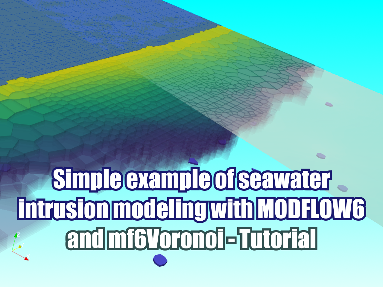
Simple example of seawater intrusion modeling with MODFLOW6 and mf6Voronoi - Tutorial
/
Evaluation of the impact from intense pumping in coastal aquifers require the simulation of variable density groundwater flow modeling since water withdrawals will produce a intrusion of seawater into the coastal aquifer. This type of modeling hasn't been widely used due to the scarcity in software tools and the evolving development of numerical codes, from the SEAWAT code to Modflow6 and Buy package.
We wanted to present seawater intrusion modeling in its more primitive form, on a simple aquifer conceptualization and aquifer geometry where the user can focus on the code implementation with MODFLOW6 - Buy package, Flopy and mf6Voronoi. We have also developed a precoded template for seawater intrusion that allows users to reduce time.
Tutorial
Code
Mesh generation
Part 1 : Voronoi mesh generation
import warnings ## Org
warnings.filterwarnings('ignore') ## Org

import os, sys ## Org
import geopandas as gpd ## Org
from mf6Voronoi.geoVoronoi import createVoronoi ## Org
from mf6Voronoi.meshProperties import meshShape ## Org
from mf6Voronoi.utils import initiateOutputFolder, getVoronoiAsShp ## Org
#Create mesh object specifying the coarse mesh and the multiplier
vorMesh = createVoronoi(meshName='seawaterIntrusion',maxRef = 250, multiplier=1.5) ## Org
#Open limit layers and refinement definition layers
vorMesh.addLimit('aquifer','../shp/modelLimit.shp') ##
vorMesh.addLayer('wellsIn','../shp/wellsStage1.shp',50) ##
vorMesh.addLayer('ref','../shp/gridRef.shp',50) ##
vorMesh.addLayer('sea','../shp/sea.shp',100) ##
vorMesh.addLayer('regGhb','../shp/regGhb.shp',50) ###Generate point pair array
vorMesh.generateOrgDistVertices() ## Org
#Generate the point cloud and voronoi
vorMesh.createPointCloud() ## Org
vorMesh.generateVoronoi() ## Org
mf6Voronoi will have a web version in 2028
Follow us: |
 |
 |
 |
 |
 |
 |
/--------Layer wellsIn discretization-------/
Progressive cell size list: [50, 125.0, 237.5] m.

/--------Layer ref discretization-------/
Progressive cell size list: [50, 125.0, 237.5] m.

/--------Layer sea discretization-------/
Progressive cell size list: [100, 250.0] m.

/--------Layer regGhb discretization-------/
Progressive cell size list: [50, 125.0, 237.5] m.

/----Sumary of points for voronoi meshing----/
Distributed points from layers: 4
Points from layer buffers: 1821
Points from max refinement areas: 78
Points from min refinement areas: 980
Total points inside the limit: 3023
/--------------------------------------------/

Time required for point generation: 0.42 seconds


/----Generation of the voronoi mesh----/

Time required for voronoi generation: 0.36 seconds
#Uncomment the next two cells if you have strong differences on discretization or you have encounter an FORTRAN error while running MODFLOW6#vorMesh.checkVoronoiQuality(threshold=0.01)#vorMesh.fixVoronoiShortSides()
#vorMesh.generateVoronoi()
#vorMesh.checkVoronoiQuality(threshold=0.01)#Export generated voronoi mesh
initiateOutputFolder('../output') ## Org
getVoronoiAsShp(vorMesh.modelDis, shapePath='../output/'+vorMesh.modelDis['meshName']+'.shp') ## OrgThe output folder ../output has been generated.
/----Generation of the voronoi shapefile----/
Time required for voronoi shapefile: 0.72 seconds# Show the resulting voronoi mesh
#open the mesh file
mesh=gpd.read_file('../output/'+vorMesh.modelDis['meshName']+'.shp') ## Org
#plot the mesh
mesh.plot(figsize=(35,25), fc='crimson', alpha=0.3, ec='teal') ## Org
Part 2 generate disv properties
# open the mesh file
mesh=meshShape('../output/'+vorMesh.modelDis['meshName']+'.shp') ## Org
# get the list of vertices and cell2d data
gridprops=mesh.get_gridprops_disv() ## OrgCreating a unique list of vertices [[x1,y1],[x2,y2],...]
100%|███████████████████████████████████████████████████████████████████████████| 3023/3023 [00:00<00:00, 15705.15it/s]
Extracting cell2d data and grid index
100%|████████████████████████████████████████████████████████████████████████████| 3023/3023 [00:01<00:00, 2722.04it/s]#create folder
initiateOutputFolder('../json') ## Org
#export disv
mesh.save_properties('../json/disvDict.json') ## OrgThe output folder ../json has been generated.Multilayer and transient model
Part 2a: generate disv properties
import sys, json, os ## Org
import rasterio, flopy ## Org
import numpy as np ## Org
import matplotlib.pyplot as plt ## Org
import geopandas as gpd ## Org
from mf6Voronoi.meshProperties import meshShape ## Org
from shapely.geometry import MultiLineString ## Org
from mf6Voronoi.tools.cellWork import getLayCellElevTupleFromRaster, getLayCellElevTupleFromElev, getLayCellElevTupleFromObs
# open the json file
with open('../json/disvDict.json') as file: ## Org
gridProps = json.load(file) ## Orgcell2d = gridProps['cell2d'] #cellid, cell centroid xy, vertex number and vertex id list
vertices = gridProps['vertices'] #vertex id and xy coordinates
ncpl = gridProps['ncpl'] #number of cells per layer
nvert = gridProps['nvert'] #number of verts
centroids=gridProps['centroids'] #cell centroids xyPart 2b: Model construction and simulation
#Extract dem values for each centroid of the voronois
from shapely.geometry import Point

src = rasterio.open('../rst/modelDem.tif')  ## Org
seaDf = gpd.read_file('../shp/sea.shp')

elevation = [] #initialize list

for centroid in centroids: #fix values of raster inside the sea polygon
    centPoint = Point(centroid) #get geometry of the cell centroid

    if centPoint.within(seaDf.iloc[0].geometry): #if it is inside the sea
        elevation.append(0)
    else:
        elevation += [x[0].item() for x in src.sample([centroid])] #assing raster value
elevation[1000:1005]
[1.0464152, 1.2116632, 1.0847379, 1.0962495, 1.1253077]nlay = 8 ## Org
mtop=np.array(elevation) #[elev[0] for i,elev in enumerate(elevation)]) ## Org
zbot=np.zeros((nlay,ncpl)) ## Org
AcuifInf_Bottom = -30# ######################### aqui me quede
zbot[0,] = AcuifInf_Bottom + (0.875 * (mtop - AcuifInf_Bottom)) ## Org
zbot[1,] = AcuifInf_Bottom + (0.75 * (mtop - AcuifInf_Bottom)) ## Org
zbot[2,] = AcuifInf_Bottom + (0.625 * (mtop - AcuifInf_Bottom)) ## Org
zbot[3,] = AcuifInf_Bottom + (0.5 * (mtop - AcuifInf_Bottom)) ## Org
zbot[4,] = AcuifInf_Bottom + (0.375 * (mtop - AcuifInf_Bottom)) ## Org
zbot[5,] = AcuifInf_Bottom + (0.25 * (mtop - AcuifInf_Bottom)) ## Org
zbot[6,] = AcuifInf_Bottom + (0.125 * (mtop - AcuifInf_Bottom)) ## Org
zbot[7,] = AcuifInf_Bottom ## OrgCreate simulation and model
# create simulation
simName = 'mf6Sim' ## Org
modelName = 'mf6Model' ## Org
modelWs = '../modelFiles' ## Org
sim = flopy.mf6.MFSimulation(sim_name=simName, version='mf6', ## Org
                             exe_name='../bin/mf6.exe', ## Org
                             continue_=True,
                             sim_ws=modelWs) ## Org
# create tdis package
tdis_rc = [(86400.0*365*50, 1, 1.0)] + [(86400*365*30, 1, 1.0)] ## 30 years, 15 years, 15 years
#tdis_rc = [(86400.0*365*50, 1, 1.0)] + [(86400*365*30, 1, 1.0) for level in range(2)] ## 30 years, 15 years, 15 years
print(tdis_rc[:3]) ## Org
tdis = flopy.mf6.ModflowTdis(sim, pname='tdis', time_units='SECONDS', ## Org
perioddata=tdis_rc, ## Org
nper=2) ## Org[(1576800000.0, 1, 1.0), (946080000, 1, 1.0)]# create gwf model
gwf = flopy.mf6.ModflowGwf(sim, ## Org
modelname=modelName, ## Org
save_flows=True, ## Org
newtonoptions="NEWTON UNDER_RELAXATION") ## Org# create iterative model solution and register the gwf model with it
imsGwf = flopy.mf6.ModflowIms(sim, ## Org
pname='ims_gwf',
complexity='COMPLEX', ## Org
outer_maximum=150, ## Org
inner_maximum=50, ## Org
outer_dvclose=0.1, ## Org
inner_dvclose=0.0001, ## Org
backtracking_number=20, ## Org
linear_acceleration='BICGSTAB') ## Org
sim.register_ims_package(imsGwf,[modelName]) ## Org# disv
disv = flopy.mf6.ModflowGwfdisv(gwf, nlay=nlay, ncpl=ncpl, ## Org
top=mtop, botm=zbot, ## Org
nvert=nvert, vertices=vertices, ## Org
cell2d=cell2d) ## Orgdisv.top.plot(figsize=(12,8), alpha=0.8) ## Org
crossSection = gpd.read_file('../shp/crossSection.shp') ## Org
sectionLine =list(crossSection.iloc[0].geometry.coords) ## Org

fig, ax = plt.subplots(figsize=(12,8)) ## Org
modelxsect = flopy.plot.PlotCrossSection(model=gwf, line={'Line': sectionLine}) ## Org
linecollection = modelxsect.plot_grid(lw=0.5) ## Org
ax.grid() ## Org
# initial conditions
ic = flopy.mf6.ModflowGwfic(gwf, strt=np.stack([mtop for i in range(nlay)])) ## Org
Kx =[7E-4 for x in range(3)] + [3E-4 for x in range(3)] + [1E-4 for x in range(2)] ## Org
icelltype = [1 for x in range(5)] + [0 for x in range(nlay - 5)] ## Org
# node property flow
npf = flopy.mf6.ModflowGwfnpf(gwf, ## Org
save_specific_discharge=True, ## Org
icelltype=icelltype, ## Org
k=Kx, ## Org
k33=np.array(Kx)/10) ## Org# define storage and transient stress periods
sto = flopy.mf6.ModflowGwfsto(gwf, ## Org
iconvert=1, ## Org
steady_state={ ## Org
0:True, ## Org
},
transient={
1:True, ## Org
},
ss=1e-06,
sy=0.001,
) ## OrgWorking with rechage, evapotranspiration
rchr = 0.2/365/86400 ## Org
rch = flopy.mf6.ModflowGwfrcha(gwf, recharge=rchr) ## Org
evtr = 1.2/365/86400 ## Org
evt = flopy.mf6.ModflowGwfevta(gwf,ievt=1,surface=mtop,rate=evtr,depth=1.0) ## Org
Definition of the intersect object
For the manipulation of spatial data to determine hydraulic parameters or boundary conditions
# Define intersection object
interIx = flopy.utils.gridintersect.GridIntersect(gwf.modelgrid) ## Org
#general boundary condition
ghbSpd = {} ## # <===== Inserted
ghbSpd[0] = [] ## # <===== Inserted
#regional flow
layCellTupleList, cellElevList = getLayCellElevTupleFromRaster(gwf,
interIx,
'../rst/waterTable.tif',
'../shp/regGhb.shp') ## # <===== Inserted
for index, layCellTuple in enumerate(layCellTupleList): ## Org
ghbSpd[0].append([layCellTuple,cellElevList[index],0.01, 0, 'regflow']) # <===== Inserted
layCellTupleList = getLayCellElevTupleFromElev(gwf,
interIx,
0,
'../shp/sea.shp',)
for layCellTuple in layCellTupleList:
ghbSpd[0].append([layCellTuple, 0, 0.20, 0, 'sea'])You have inserted a fixed elevationghb = flopy.mf6.ModflowGwfghb(gwf, stress_period_data=ghbSpd, auxiliary=['CONCENTRATION'], boundnames=True) ## <==== modified
# Observation package for Drain
obsDict = { # <===== Inserted
"{}.ghb.obs.csv".format(modelName): [ # <===== Inserted
("regflow", "ghb", "regionalFlow"), # <===== Inserted
("sea", "ghb", "sea") # <===== Inserted
] # <===== Inserted
} # <===== Inserted
# Attach observation package to DRN package
ghb.obs.initialize( # <===== Inserted
filename=gwf.name+".ghb.obs", # <===== Inserted
digits=10, # <===== Inserted
print_input=True, # <===== Inserted
continuous=obsDict # <===== Inserted
) # <===== Inserted#define buy package
buyModName = 'modelBuy'
Csalt = 35.
Cfresh = 0.
densesalt = 1025.
densefresh = 1000.
denseslp = (densesalt - densefresh) / (Csalt - Cfresh)
pd = [(0, denseslp, 0., buyModName, 'CONCENTRATION')]
buy = flopy.mf6.ModflowGwfbuy(gwf, denseref=1000., nrhospecies=1,packagedata=pd)#ghb plot
ghb.plot(mflay=0, kper=0) # <===== Inserted
from copy import copy
#well bc

wellSpd = {} ## # <===== Inserted
wellSpd[0] = [] ## # <===== Inserted
wellSpd[1] = []

#regional flow
# from raster
# layCellTupleList, cellElevList = getLayCellElevTupleFromRaster(gwf,
#                                                                interIx,
#                                                                '../rst/modelDemMinus45.tif',
#                                                                '../shp/wellsStage1.shp') ## # <===== Inserted

# for index, layCellTuple in enumerate(layCellTupleList): ## Org
#     wellSpd[1].append([layCellTuple,-0.01,'wellsStage1']) # <===== Inserted

# from elevation
layCellTupleList = getLayCellElevTupleFromElev(gwf,
                                               interIx,
                                               -20,
                                               '../shp/wellsStage1.shp',)
for layCellTuple in layCellTupleList:
    wellSpd[1].append([layCellTuple, -0.005, 'wellsStage1'])

wellSpd[1][:10]
You have inserted a fixed elevation
[[(5, 1784), -0.005, 'wellsStage1'],
[(5, 2561), -0.005, 'wellsStage1'],
[(5, 2713), -0.005, 'wellsStage1'],
[(5, 1468), -0.005, 'wellsStage1'],
[(5, 1179), -0.005, 'wellsStage1'],
[(5, 2523), -0.005, 'wellsStage1'],
[(5, 983), -0.005, 'wellsStage1'],
[(5, 2252), -0.005, 'wellsStage1'],
[(5, 1240), -0.005, 'wellsStage1'],
[(5, 2293), -0.005, 'wellsStage1']]wel = flopy.mf6.ModflowGwfwel(gwf, stress_period_data=wellSpd, boundnames=True) ## <==== modified
# Observation package for Drain
obsDict = { # <===== Inserted
"{}.wel.obs.csv".format(modelName): [ # <===== Inserted
("wellsStage1", "wel", "wellsStage1") # <===== Inserted
] # <===== Inserted
} # <===== Inserted
# Attach observation package to DRN package
wel.obs.initialize( # <===== Inserted
filename=gwf.name+".wel.obs", # <===== Inserted
digits=10, # <===== Inserted
print_input=True, # <===== Inserted
continuous=obsDict # <===== Inserted
) # <===== Inserted
#ghb plot
wel.plot(mflay=5, kper=1) # <===== Inserted
from copy import copy
#well bc

wellSpd = {} ## # <===== Inserted
wellSpd[0] = [] ## # <===== Inserted
wellSpd[1] = []

#regional flow
# from raster
# layCellTupleList, cellElevList = getLayCellElevTupleFromRaster(gwf,
#                                                                interIx,
#                                                                '../rst/modelDemMinus45.tif',
#                                                                '../shp/wellsStage1.shp') ## # <===== Inserted

# for index, layCellTuple in enumerate(layCellTupleList): ## Org
#     wellSpd[1].append([layCellTuple,-0.01,'wellsStage1']) # <===== Inserted

# from elevation
layCellTupleList = getLayCellElevTupleFromElev(gwf,
                                               interIx,
                                               -20,
                                               '../shp/wellsStage1.shp',)
for layCellTuple in layCellTupleList:
    wellSpd[1].append([layCellTuple, -0.005, 'wellsStage1'])

wellSpd[1][:10]
You have inserted a fixed elevation
[[(5, 1784), -0.005, 'wellsStage1'],
[(5, 2561), -0.005, 'wellsStage1'],
[(5, 2713), -0.005, 'wellsStage1'],
[(5, 1468), -0.005, 'wellsStage1'],
[(5, 1179), -0.005, 'wellsStage1'],
[(5, 2523), -0.005, 'wellsStage1'],
[(5, 983), -0.005, 'wellsStage1'],
[(5, 2252), -0.005, 'wellsStage1'],
[(5, 1240), -0.005, 'wellsStage1'],
[(5, 2293), -0.005, 'wellsStage1']]wel = flopy.mf6.ModflowGwfwel(gwf, stress_period_data=wellSpd, boundnames=True) ## <==== modified
# Observation package for Drain
obsDict = { # <===== Inserted
"{}.wel.obs.csv".format(modelName): [ # <===== Inserted
("wellsStage1", "wel", "wellsStage1") # <===== Inserted
] # <===== Inserted
} # <===== Inserted
# Attach observation package to DRN package
wel.obs.initialize( # <===== Inserted
filename=gwf.name+".wel.obs", # <===== Inserted
digits=10, # <===== Inserted
print_input=True, # <===== Inserted
continuous=obsDict # <===== Inserted
) # <===== Inserted
#ghb plot
wel.plot(mflay=5, kper=1) # <===== Inserted[<Axes: title={'center': ' wel_0 location stress period 2 layer 6'}>]
Define transport model
#create transport package
gwt = flopy.mf6.ModflowGwt(sim, modelname=buyModName)

#register solver for transport model
imsGwt = flopy.mf6.ModflowIms(sim,
                              pname='ims_gwt',
                              #print_option='SUMMARY', ## Org
                              outer_dvclose=2e-4, ## Org
                              inner_dvclose=3e-4, ## Org
                              linear_acceleration='BICGSTAB') ## Org
sim.register_ims_package(imsGwt,[gwt.name])

#define spatial discretization
gwtDisv = flopy.mf6.ModflowGwtdisv(gwt, nlay=disv.nlay.data,
                                   ncpl=disv.ncpl.data,
                                   nvert=disv.nvert.data,
                                   top=disv.top.data,
                                   botm=disv.botm.data,
                                   vertices=disv.vertices.array.tolist(),
                                   cell2d=disv.cell2d.array.tolist(),
                                  )
## Org
sim.register_ims_package(imsGwf,[modelName])
#sim.write_simulation()#define starting concentrations
strtConc = np.zeros((disv.nlay.data, disv.ncpl.data), dtype=np.float32)
ghbList = ghb.stress_period_data.array[0].tolist()
ghbList[-5:][((0, 736), 0.0, 0.2, 0, 'sea'),
((0, 737), 0.0, 0.2, 0, 'sea'),
((0, 739), 0.0, 0.2, 0, 'sea'),
((0, 740), 0.0, 0.2, 0, 'sea'),
((0, 758), 0.0, 0.2, 0, 'sea')]for ghbItem in ghbList:
if ghbItem[4] == 'sea':
strtConc[:,ghbItem[0][1]] = 35 #apply for all layers below the ghb
gwtIc = flopy.mf6.ModflowGwtic(gwt, strt=strtConc)# create plot of initial concentratios
fig = plt.figure(figsize=(12, 12))
ax = fig.add_subplot(1, 1, 1, aspect = 'equal')
mapview = flopy.plot.PlotMapView(model=gwf,layer = 1)
plot_array = mapview.plot_array(strtConc,masked_values=[-1e+30], cmap=plt.cm.summer)
plt.colorbar(plot_array, shrink=0.75,orientation='horizontal', pad=0.08, aspect=50)
#define advection
adv = flopy.mf6.ModflowGwtadv(gwt, scheme='UPSTREAM')
#define dispersion
dsp = flopy.mf6.ModflowGwtdsp(gwt,alh=10,ath1=10)
#define mobile storage and transfer
porosity = 0.30
sto = flopy.mf6.ModflowGwtmst(gwt, porosity=porosity)
#define sink and source package
sourcerecarray = ['GHB_0','AUX','CONCENTRATION']
ssm = flopy.mf6.ModflowGwtssm(gwt, sources=sourcerecarray)
#define constant concentration package
cncSp = []
for row in ghb.stress_period_data.array[0]:
if row['boundname'] == 'sea':
cncSp.append([row[0],35])
cncSpd = {0:cncSp,1:cncSp}
cnc = flopy.mf6.ModflowGwtcnc(gwt,stress_period_data=cncSpd)
# cnc.plot(mflay=0, lw=0.1, figsize=(12,12))#working with observation points
obsList = []
nameList, obsLayCellList = getLayCellElevTupleFromObs(gwf, ## Org
interIx, ## Org
'../shp/obsPoints.shp', ## Org
'name', ## Org
'elev') ## Org
for obsName, obsLayCell in zip(nameList, obsLayCellList): ## Org
obsList.append((obsName,'concentration',obsLayCell[0]+1,obsLayCell[1]+1)) ## Org
obs = flopy.mf6.ModflowUtlobs( ## Org
gwt,
filename=gwt.name+'.obs', ## Org
digits=10, ## Org
print_input=True, ## Org
continuous={gwt.name+'.obs.csv': obsList} ## Org
)Working for cell 1468
Well screen elev of -20.00 found at layer 5
Working for cell 983
Well screen elev of -20.00 found at layer 5
Working for cell 1627
Well screen elev of -20.00 found at layer 5
Working for cell 1865
Well screen elev of -20.00 found at layer 5Set the output control and exchange / run model
#oc for flow
head_filerecord = f"{gwf.name}.hds" ## Org
budget_filerecord = f"{gwf.name}.cbc" ## Org
oc = flopy.mf6.ModflowGwfoc(gwf, ## Org
                            head_filerecord=head_filerecord, ## Org
                            budget_filerecord = budget_filerecord, ## Org
                            saverecord=[("HEAD", "LAST"),("BUDGET","LAST")]) ## Org

#oc for transport
oc = flopy.mf6.ModflowGwtoc(gwt,
                            concentration_filerecord=buyModName+'.ucn',
                            saverecord=[('CONCENTRATION', 'ALL')])

#define model flow and transport exchange
name = 'modelExchange'
gwfgwt = flopy.mf6.ModflowGwfgwt(sim, exgtype='GWF6-GWT6',
                                 exgmnamea=gwf.name, exgmnameb=buyModName,
                                 filename='{}.gwfgwt'.format(name))
# Run the simulation
sim.write_simulation() ## Orgwriting simulation...
writing simulation name file...
writing simulation tdis package...
writing solution package ims_gwt...
writing solution package ims_gwf...
writing package modelExchange.gwfgwt...
writing model mf6Model...
writing model name file...
writing package disv...
writing package ic...
writing package npf...
writing package sto...
writing package rcha_0...
writing package evta_0...
writing package ghb_0...
INFORMATION: maxbound in ('gwf6', 'ghb', 'dimensions') changed to 787 based on size of stress_period_data
writing package obs_0...
writing package buy...
writing package wel_0...
INFORMATION: maxbound in ('gwf6', 'wel', 'dimensions') changed to 45 based on size of stress_period_data
writing package obs_1...
writing package oc...
writing model modelBuy...
writing model name file...
writing package disv...
writing package ic...
writing package adv...
writing package dsp...
writing package mst...
writing package ssm...
writing package cnc_0...
INFORMATION: maxbound in ('gwt6', 'cnc', 'dimensions') changed to 724 based on size of stress_period_data
writing package obs_0...
writing package oc...success, buff = sim.run_simulation() ## OrgFloPy is using the following executable to run the model: ..\bin\mf6.exe
MODFLOW 6
U.S. GEOLOGICAL SURVEY MODULAR HYDROLOGIC MODEL
VERSION 6.6.0 12/20/2024
MODFLOW 6 compiled Dec 31 2024 17:10:16 with Intel(R) Fortran Intel(R) 64
Compiler Classic for applications running on Intel(R) 64, Version 2021.7.0
Build 20220726_000000
This software has been approved for release by the U.S. Geological
Survey (USGS). Although the software has been subjected to rigorous
review, the USGS reserves the right to update the software as needed
pursuant to further analysis and review. No warranty, expressed or
implied, is made by the USGS or the U.S. Government as to the
functionality of the software and related material nor shall the
fact of release constitute any such warranty. Furthermore, the
software is released on condition that neither the USGS nor the U.S.
Government shall be held liable for any damages resulting from its
authorized or unauthorized use. Also refer to the USGS Water
Resources Software User Rights Notice for complete use, copyright,
and distribution information.
MODFLOW runs in SEQUENTIAL mode
Run start date and time (yyyy/mm/dd hh:mm:ss): 2025/10/21 10:23:21
Writing simulation list file: mfsim.lst
Using Simulation name file: mfsim.nam
Solving: Stress period: 1 Time step: 1
Solving: Stress period: 2 Time step: 1
Run end date and time (yyyy/mm/dd hh:mm:ss): 2025/10/21 10:23:27
Elapsed run time: 5.127 Seconds
Normal termination of simulation.Model output visualization
headObj = gwf.output.head() ## Org
headObj.get_kstpkper() ## Org
[(np.int32(0), np.int32(0)), (np.int32(0), np.int32(1))]kper = 1 ## Org
lay = 0 ## Orgheads = headObj.get_data(kstpkper=(0,kper))
#heads[lay,0,:5]
#heads = headObj.get_data(kstpkper=(0,0))
#np.save('npy/headCalibInitial', heads)### Plot the heads for a defined layer and boundary conditions
fig = plt.figure(figsize=(12,8)) ## Org
ax = fig.add_subplot(1, 1, 1, aspect='equal') ## Org
modelmap = flopy.plot.PlotMapView(model=gwf) ## Org
####
levels = np.linspace(heads[heads>-1e+30].min(),heads[heads>-1e+30].max(),num=50) ## Org
contour = modelmap.contour_array(heads[lay],ax=ax,levels=levels,cmap='PuBu')
ax.clabel(contour) ## Org
quadmesh = modelmap.plot_bc('GHB') ## Org
cellhead = modelmap.plot_array(heads[lay],ax=ax, cmap='Blues', alpha=0.8)
linecollection = modelmap.plot_grid(linewidth=0.3, alpha=0.5, color='cyan', ax=ax) ## Org
plt.colorbar(cellhead, shrink=0.75) ## Org
plt.show() ## Org
crossSection = gpd.read_file('../shp/crossSection.shp')
sectionLine =list(crossSection.iloc[0].geometry.coords)

waterTable = flopy.utils.postprocessing.get_water_table(heads)

fig, ax = plt.subplots(figsize=(12,8))
xsect = flopy.plot.PlotCrossSection(model=gwf, line={'Line': sectionLine})
lc = xsect.plot_grid(lw=0.5)
xsect.plot_array(heads, alpha=0.5)
xsect.plot_surface(waterTable)
xsect.plot_bc('ghb', kper=kper, facecolor='none', edgecolor='teal')
plt.show()
Explore the concentration results
concObj = gwt.output.concentration() ## Org
concObj.get_kstpkper() ## Org
[(np.int32(0), np.int32(0)), (np.int32(0), np.int32(1))]#define time series and stress period to plot
ts = (0,0)
#get concentrations for the time step
tempConc = concObj.get_data(kstpkper=ts)### Review the flow model
fig = plt.figure(figsize=(12, 12))
ax = fig.add_subplot(1, 1, 1, aspect = 'equal')
mapview = flopy.plot.PlotMapView(model=gwf,layer = 4)
plot_array = mapview.plot_array(tempConc,masked_values=[-1e+30], cmap=plt.cm.summer)
plt.colorbar(plot_array, shrink=0.75,orientation='horizontal', pad=0.08, aspect=50)
### Zoom to intrusion
# fig = plt.figure(figsize=(12, 12))
# ax = fig.add_subplot(1, 1, 1, aspect = 'equal')
# mapview = flopy.plot.PlotMapView(model=gwf,layer = 4)

# plot_array = mapview.plot_array(tempConc,masked_values=[-1e+30], cmap=plt.cm.summer)
# plt.colorbar(plot_array, shrink=0.75,orientation='horizontal', pad=0.08, aspect=50)
# ax.set_xlim(200000,206000)
# ax.set_ylim(8798000,8803000)
#plot heads on line
tempHead = headObj.get_data(kstpkper=ts)
fig, ax = plt.subplots(figsize=(18,6))
crossSection = gpd.read_file('../shp/crossSection.shp')
sectionLine =list(crossSection.iloc[0].geometry.coords)
crossview = flopy.plot.PlotCrossSection(model=gwf, line={"line": sectionLine})
crossview.plot_grid(alpha=0.25)
strtArray = crossview.plot_array(tempConc, masked_values=[1e30], cmap=plt.cm.summer)
cb = plt.colorbar(strtArray, shrink=0.5)
3d geometry generation on Vtk format
#Vtk generation
import flopy ## Org
from mf6Voronoi.tools.vtkGen import Mf6VtkGenerator ## Org
from mf6Voronoi.utils import initiateOutputFolder ## Org
# load simulation
simName = 'mf6Sim' ## Org
modelName = 'mf6Model' ## Org
modelWs = '../modelFiles' ## Org
sim = flopy.mf6.MFSimulation.load(sim_name=modelName, version='mf6', ## Org
exe_name='bin/mf6.exe', ## Org
sim_ws=modelWs) ## Orgloading simulation...
loading simulation name file...
loading tdis package...
loading model gwf6...
loading package disv...
loading package ic...
loading package npf...
loading package sto...
loading package rch...
loading package evt...
loading package ghb...
loading package buy...
loading package wel...
loading package oc...
loading model gwt6...
loading package disv...
loading package ic...
loading package adv...
loading package dsp...
loading package mst...
loading package ssm...
loading package cnc...
loading package obs...
loading package oc...
loading exchange package gwf-gwt_exg_0...
loading solution package mf6model...
loading solution package modelbuy...vtkDir = '../vtk' ## Org
initiateOutputFolder(vtkDir) ## Org
mf6Vtk = Mf6VtkGenerator(sim, vtkDir) ## OrgThe output folder ../vtk exists and has been clearedbuild faster, analyze more
Follow us: |
|
|
|
|
|
|
/---------------------------------------/

The Vtk generator engine has been started

/---------------------------------------/
#list models on the simulation
mf6Vtk.listModels() ## OrgModels in simulation: ['mf6model', 'modelbuy']mf6Vtk.loadModel(modelName) ## OrgPackage list: ['DISV', 'IC', 'NPF', 'STO', 'RCHA_0', 'EVTA_0', 'GHB_OBS', 'GHB_0', 'BUY', 'WEL_OBS', 'WEL_0', 'OC']#show output data
headObj = mf6Vtk.gwf.output.head() ## Org
headObj.get_kstpkper() ## Org[(np.int32(0), np.int32(0)), (np.int32(0), np.int32(1))]#generate model geometry as vtk and parameter array
mf6Vtk.generateGeometryArrays() ## Org#generate parameter vtk
mf6Vtk.generateParamVtk() ## OrgParameter Vtk Generated#generate bc and obs vtk
mf6Vtk.generateBcObsVtk(nper=1) ## Org/--------RCHA_0 vtk generation-------/
Working for RCHA_0 package, creating the datasets: dict_keys(['irch', 'recharge', 'aux'])
[WARNING] There is no data for the required stress period
Vtk file took 0.0144 seconds to be generated.
/--------RCHA_0 vtk generated-------/
/--------EVTA_0 vtk generation-------/
Working for EVTA_0 package, creating the datasets: dict_keys(['ievt', 'surface', 'rate', 'depth', 'aux'])
[WARNING] There is no data for the required stress period
Vtk file took 0.0044 seconds to be generated.
/--------EVTA_0 vtk generated-------/
/--------GHB_0 vtk generation-------/
Working for GHB_0 package, creating the datasets: ('bhead', 'cond', 'concentration', 'boundname')
[WARNING] There is no data for the required stress period
Vtk file took 0.0174 seconds to be generated.
/--------GHB_0 vtk generated-------/
/--------WEL_0 vtk generation-------/
Working for WEL_0 package, creating the datasets: ('q', 'boundname')
Vtk file took 0.0589 seconds to be generated.
/--------WEL_0 vtk generated-------/mf6Vtk.generateHeadVtk(nper=1, crop=True) ## Orgmf6Vtk.generateWaterTableVtk(nper=1) ## Orggwt = sim.get_model('modelbuy')
concObj = gwt.output.concentration()
concObj.get_times()[np.float64(1576800000.0), np.float64(2522880000.0)]conc = concObj.get_data(totim=2522880000.0)
conc[4][0]array([3.49999990e+01, 3.49999995e+01, 3.49999997e+01, ...,
9.46436088e-34, 8.36667681e-34, 8.49161843e-34])mf6Vtk.generateArrayVtk(conc, 'conc80y', nper=1,nstp=0, crop=True)Input data
You can download the input data from this link:
owncloud.hatarilabs.com/s/RJhd1QPfvpD73HB
Password: Hatarilabs