Surface analysis at regional level requires a higher degree of calculation to assess several topics of land management. Usually those types of analysis over raster files were limited to GIS desktop software with results for a single raster and with limited options to create pixel value charts.

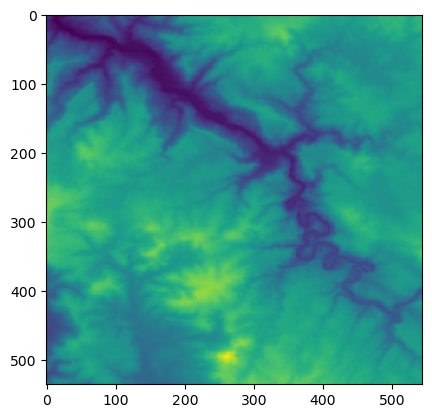
Python, Rasterio, Landlab and other high performance packages allow us to have another view of our surface elevation and evaluate different variables that were unthinkable over traditional GIS software. This tutorial shows the complete procedure to open a raster file with Rasterio, import as a Landlab model grid, fill sink and calculate the drainage area. Finally from the Landlab results a dataframe was constructed and the drainage areas were classified in intervals to be plotted on a boxplot with the steepest slope.

Tutorial

Input data

You can download the input data from this link.

Code

# import generic packages
import numpy as np
from matplotlib import pyplot as plt
import pandas as pd

# import geospatial packages
import rasterio
from rasterio.plot import show

# import landlab components
from landlab import RasterModelGrid, imshow_grid
from landlab.components import (
    DepressionFinderAndRouter,
    FlowAccumulator
)

#open raster image 
rasterObj = rasterio.open('../rst/clippedDem_12N.tif')
show(rasterObj)

<Axes: >

#extract array from raster
elevArray = rasterObj.read(1)
plt.imshow(elevArray)

<matplotlib.image.AxesImage at 0x1b7f41183a0>

#show array
elevArray

array([[1475, 1470, 1467, ..., 1809, 1809, 1808],
       [1469, 1464, 1460, ..., 1816, 1816, 1816],
       [1461, 1458, 1453, ..., 1815, 1819, 1820],
       ..., 
       [1618, 1616, 1616, ..., 1752, 1753, 1754],
       [1621, 1617, 1617, ..., 1743, 1745, 1749],
       [1621, 1617, 1617, ..., 1739, 1740, 1743]], dtype=int16)

#create grid from raster attributes
nrows = rasterObj.height  # number of raster cells on each side, initially 150
ncols = rasterObj.width
dxy = rasterObj.transform.a  # side length of a raster model cell, or resolution [m], initially 50

# define a landlab raster
mg = RasterModelGrid(shape=(nrows, ncols), 
                     xy_spacing=dxy,
                     xy_of_lower_left=(rasterObj.bounds[0],rasterObj.bounds[1]))

# create a dataset of zero values
zr = mg.add_zeros("topographic__elevation", at="node")
imshow_grid(mg, "topographic__elevation", shrink=0.5)

# apply cell elevation to defined arrray
zr += elevArray[::-1,:].ravel()
imshow_grid(mg, "topographic__elevation", shrink=0.5)

#run the component to accumulate flow and calculate area
fr = FlowAccumulator(mg, flow_director='D8')
fr.run_one_step()

#show the partial drainage area and check uncontinours streams
imshow_grid(mg, 'drainage_area', shrink=0.5)

#fill sinks
df = DepressionFinderAndRouter(mg)
df.map_depressions()

#plot corrected drainage area
fig = plt.figure(figsize=(12,6))
imshow_grid(mg, 'drainage_area', shrink=0.5)

#create a pandas dataframe for boxplot
dfMg = pd.DataFrame(columns=['slope','area(Ha)'])
dfMg['slope']=mg.at_node["topographic__steepest_slope"][mg.core_nodes]
dfMg['area(Ha)']=mg.at_node["drainage_area"][mg.core_nodes]/10000
dfMg.head()

	slope	area(Ha)
0	0.038986	0.065793
1	0.303241	0.065793
2	0.545807	0.065793
3	0.467834	0.065793
4	0.389862	0.065793

#create interval an apply into a new columns
areaInterval = pd.interval_range(0,dfMg['area(Ha)'].max()//100*100,25)
dfMg['areaInterval(Ha)'] = pd.cut(dfMg['area(Ha)'], bins=areaInterval)
dfMg.head()

	slope	area(Ha)	areaInterval(Ha)
0	0.038986	0.065793	(0.0, 580.0]
1	0.303241	0.065793	(0.0, 580.0]
2	0.545807	0.065793	(0.0, 580.0]
3	0.467834	0.065793	(0.0, 580.0]
4	0.389862	0.065793	(0.0, 580.0]

#plot the graph of maximum slope vs drainage area 
fig, ax = plt.subplots(figsize=(12, 6))
dfMg.boxplot('slope', by='areaInterval(Ha)', ax=ax, rot=90)
#ax.set_yscale('log')
ax.set_ylim(-0.01,0.8)