Spatial analysis is such an interesting discipline because it allows the evaluation of every phenomena related to their location. However, for some parts of the data processing the workflow on a GIS Graphical Computer Interface (GUI) can be repetitive and time consuming. Researchers need better and more efficient tools to process more amount of data in less amount of time and even with less quantity of software tools.

We have create a innovative script to generate an elevation raster file from a contour line with several steps of data processing. The script recognizes invalid geometries, simplify the polylines and extract vertices while creates a point geodataframe that is interpolated and geotransformed as a geospatial raster in .tiff format.

Tutorial

Python script

Geopandas geodataframes generation

%matplotlib inline
import geopandas as gpd
import pandas as pd
import matplotlib.pyplot as plt
from shapely.geometry import Point, Polygon
from shapely.ops import split

#Shapefile list
%ls ..\Shp\*.shp

El volumen de la unidad C no tiene etiqueta.
 El n£mero de serie del volumen es: 24E6-96EB

 Directorio de C:\Users\GIDAWK1\Documents\howToCreateAreaofInterestRasterfromContourLineswithPythonandGeopandas\Shp

27/11/2019  09:43 a.m.         7,667,184 contours_10m.shp
29/11/2019  10:51 a.m.         7,436,972 contours_10m_v2.shp
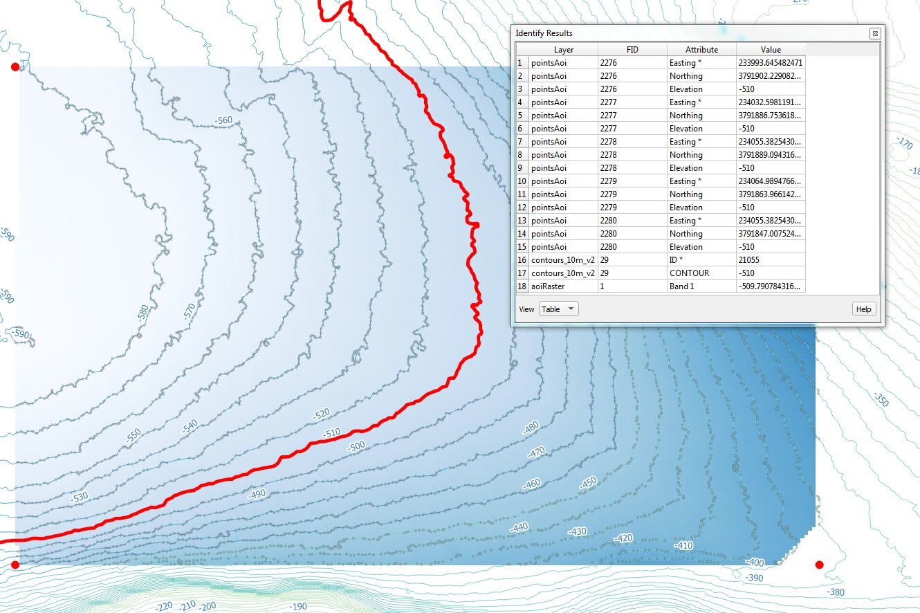
02/12/2019  03:08 p.m.           187,336 pointsAoi.shp
02/12/2019  11:44 a.m.               236 rasterAoi.shp
               4 archivos     15,291,728 bytes
               0 dirs  28,501,250,048 bytes libres

#Open countour lines and area of interest
topo1 = gpd.read_file('../Shp/contours_10m_v2.shp')
rasterAoi = gpd.read_file('../Shp/rasterAoi.shp')
aoiGeom = rasterAoi.loc[0].geometry
topo1.crs

{'init': 'epsg:32611'}

#Plot of the countour line with the selected area to extract vertices
ax = rasterAoi.plot(color='green', figsize=(12,12), alpha=0.2);
topo1.plot(ax=ax,alpha=0.5)
ax.grid()

Vertex extraction to the Area of Interest

compDf = gpd.GeoDataFrame()
compDf['geometry']=None
i=0

for index, row in topo1.iterrows():
    #index counter
    if index % 100 == 0:
        print('Processing polylines_'+str(index)+'\n')

    if row.geometry!=None: #Check for false geometries
        try:          
            if row.geometry.disjoint(aoiGeom)==False: #Filter all lines that dont cross the polygon 
                #print(len(row.geometry.coords))
                simpRow = row.geometry.simplify(5,preserve_topology=True)
                vertexBefore = len(row.geometry.coords)
                vertexAfter = len(simpRow.coords)
                reductionPercen = vertexAfter/vertexBefore*100

                print('Vertex before: %d, Vertex after: %d, Reduction rate: %.2f'%(vertexBefore,vertexAfter,reductionPercen))
                for coord in simpRow.coords:
                    if Point(coord).within(aoiGeom): #Check if vertex is inside the polygon
                        compDf.loc[i]=str(row.ID) #Assign values to the dataframe
                        compDf.loc[i,'Easting']=coord[0]
                        compDf.loc[i,'Northing']=coord[1]
                        compDf.loc[i,'Elevation']=row.CONTOUR
                        compDf.loc[i,'geometry']=Point(coord)
                        i+=1

                        #Counter of proccessed points
                        if i % 1000 == 0:
                            print('Processed Vertices_'+str(i))                    
        except ValueError: pass

compDf.head()

Processing polylines_0

Vertex before: 81, Vertex after: 48, Reduction rate: 59.26
Vertex before: 1888, Vertex after: 1035, Reduction rate: 54.82
Vertex before: 2111, Vertex after: 1049, Reduction rate: 49.69
Vertex before: 2486, Vertex after: 1229, Reduction rate: 49.44
Vertex before: 2665, Vertex after: 1291, Reduction rate: 48.44
Processed Vertices_1000
Vertex before: 2721, Vertex after: 1288, Reduction rate: 47.34
Vertex before: 2828, Vertex after: 1286, Reduction rate: 45.47
Vertex before: 3056, Vertex after: 1306, Reduction rate: 42.74
Processed Vertices_2000
Vertex before: 3093, Vertex after: 1324, Reduction rate: 42.81
Vertex before: 3480, Vertex after: 1475, Reduction rate: 42.39
Vertex before: 3893, Vertex after: 1655, Reduction rate: 42.51
Processed Vertices_3000
Vertex before: 3111, Vertex after: 1275, Reduction rate: 40.98
Vertex before: 3654, Vertex after: 1398, Reduction rate: 38.26
Vertex before: 3558, Vertex after: 1216, Reduction rate: 34.18
Vertex before: 3612, Vertex after: 1294, Reduction rate: 35.83
Processed Vertices_4000
Vertex before: 3606, Vertex after: 1283, Reduction rate: 35.58
Vertex before: 3674, Vertex after: 1226, Reduction rate: 33.37
Vertex before: 3723, Vertex after: 1268, Reduction rate: 34.06
Vertex before: 3796, Vertex after: 1290, Reduction rate: 33.98
Processed Vertices_5000
Vertex before: 3832, Vertex after: 1293, Reduction rate: 33.74
Vertex before: 3838, Vertex after: 1207, Reduction rate: 31.45
Vertex before: 4043, Vertex after: 1247, Reduction rate: 30.84
Vertex before: 4121, Vertex after: 1259, Reduction rate: 30.55
Vertex before: 4177, Vertex after: 1252, Reduction rate: 29.97
Processed Vertices_6000
Vertex before: 4293, Vertex after: 1245, Reduction rate: 29.00
Vertex before: 4399, Vertex after: 1310, Reduction rate: 29.78
Vertex before: 4367, Vertex after: 1242, Reduction rate: 28.44
Vertex before: 4435, Vertex after: 1259, Reduction rate: 28.39
Vertex before: 4490, Vertex after: 1266, Reduction rate: 28.20
Vertex before: 4525, Vertex after: 1316, Reduction rate: 29.08
Vertex before: 4616, Vertex after: 1367, Reduction rate: 29.61
Vertex before: 4679, Vertex after: 1349, Reduction rate: 28.83
Vertex before: 4857, Vertex after: 1445, Reduction rate: 29.75
Vertex before: 4945, Vertex after: 1489, Reduction rate: 30.11
Vertex before: 5242, Vertex after: 1620, Reduction rate: 30.90
Vertex before: 5754, Vertex after: 1666, Reduction rate: 28.95
Vertex before: 6588, Vertex after: 1929, Reduction rate: 29.28
Processing polylines_100

Processing polylines_200

Processing polylines_300

	geometry	Easting	Northing	Elevation
0	POINT (222455.383 3788700.041)	222455	3.7887e+06	-590
1	POINT (222411.465 3788720.048)	222411	3.78872e+06	-590
2	POINT (222401.342 3788809.926)	222401	3.78881e+06	-590
3	POINT (222355.383 3788845.643)	222355	3.78885e+06	-590
4	POINT (222255.383 3788803.316)	222255	3.7888e+06	-590

#Representation of the extracted vertices and the area of interest
ax = rasterAoi.plot(color='green', figsize=(12,12), alpha=0.2);
topo1.plot(ax=ax,color='cyan',alpha=0.5)
compDf.plot(ax=ax,alpha=0.5)
ax.grid()

#Export point to shapefile
compDf.crs={'init': 'epsg:32611'}
compDf.to_file('../Shp/pointsAoi.shp')

Point interpolation

import numpy as np
from scipy.interpolate import griddata

#From the dataFrame
points = compDf[['Easting','Northing']].values
values = compDf['Elevation'].values

#Assign the raster resoulution
rasterRes = 100.0

#Get the Area of Interest dimensions and number of rows / cols
print(aoiGeom.bounds)
xDim = aoiGeom.bounds[2]-aoiGeom.bounds[0]
yDim = aoiGeom.bounds[3]-aoiGeom.bounds[1]
print('Raster X Dim: %.2f, Raster Y Dim: %.2f'%(xDim,yDim))
nCols = xDim / rasterRes
nRows = yDim / rasterRes
print('Number of cols:  %.2f, Number of rows: %.2f'%(nCols,nRows)) #Check if the cols and row don't have decimals

(222000.0, 3783000.0, 243000.0, 3796000.0)
Raster X Dim: 21000.00, Raster Y Dim: 13000.00
Number of cols:  210.00, Number of rows: 130.00

#We create an array on the cell centroid
grid_y, grid_x = np.mgrid[aoiGeom.bounds[1]+rasterRes/2:aoiGeom.bounds[3]-rasterRes/2:nRows*1j,
                         aoiGeom.bounds[0]+rasterRes/2:aoiGeom.bounds[2]+rasterRes/2:nCols*1j]

mtop = griddata(points, values, (grid_x, grid_y), method='cubic')
mtop[:5,:5]

array([[          nan, -480.77331   , -480.06521355, -479.63126685,
        -480.03963447],
       [          nan, -485.85168813, -484.67218837, -484.55962848,
        -483.67878073],
       [          nan, -491.72186276, -490.12375354, -491.89022442,
        -491.8011287 ],
       [          nan, -498.59717162, -498.41920838, -497.27970783,
        -497.03388778],
       [          nan, -504.09576321, -504.01128831, -501.76031806,
        -500.74936978]])

import matplotlib.pyplot as plt
plt.imshow(mtop)
plt.colorbar()

<matplotlib.colorbar.Colorbar at 0xeaaafd0>

Raster generation

from osgeo import gdal, gdal_array, osr

geotransform = [aoiGeom.bounds[0],rasterRes,0,aoiGeom.bounds[1],0,rasterRes] #[xmin,xres,0,ymax,0,-yres]
raster = gdal.GetDriverByName('GTiff').Create("../Rst/aoiRaster.tif",int(nCols),int(nRows),1,gdal.GDT_Float64)
raster.SetGeoTransform(geotransform)

srs=osr.SpatialReference()
srs.ImportFromEPSG(32611)

raster.SetProjection(srs.ExportToWkt())
raster.GetRasterBand(1).WriteArray(mtop)
del raster