Large amount of spatial data is indexed and delivered through files in Hierarchical Data Format (HDF). These files are compatible with desktop GIS software as QGIS but they are not so easy to open/read/process with standard Python libraries as Rasterio, or with dedicated libraries. On our research we found the spatial functionality on the powerful GDAL binaries and library for Python.

We have done an applied case for the download, reproject (to WGS84) and clip to the area of interest of several MYD16A2 actual evapotranspiration images. We have also create an interactive visualization of the clipped images that allow us to examine the precipitation trends and the challenges in the use of these data products.

For this tutorial you need:

1. Windows Subsytem for Linux (WSL) in your computer:

On Powershell please check: wsl --status

If you dont have it installed please type: wsl --install

2. An account in NASA earthdata:

urs.earthdata.nasa.gov/users/new

Animation

Final representation of the translated and clipped evapotransporation images:

Tutorial

Python code

Code for downloading data:

#!pip install earthaccess

import earthaccess
auth = earthaccess.login()

We are already authenticated with NASA EDL

#earthaccess.search_data?

results = earthaccess.search_data(
    short_name='MYD16A2',
    cloud_hosted=True,
    bounding_box=(-77.6, -9.9, -76.9, -9.2),
    temporal=("2021-01-01", "2021-12-31"),
    count=10
)

Granules found: 46

# if the data set is cloud hosted there will be S3 links available. The access parameter accepts "direct" or "external", direct access is only possible if you are in the us-west-2 region in the cloud.
data_links = [granule.data_links(access="direct") for granule in results]

data_links[:10]

[['s3://lp-prod-protected/MYD16A2.061/MYD16A2.A2021001.h10v09.061.2021067224124/MYD16A2.A2021001.h10v09.061.2021067224124.hdf'],
 ['s3://lp-prod-protected/MYD16A2.061/MYD16A2.A2021009.h10v09.061.2021068070135/MYD16A2.A2021009.h10v09.061.2021068070135.hdf'],
 ['s3://lp-prod-protected/MYD16A2.061/MYD16A2.A2021017.h10v09.061.2021068143354/MYD16A2.A2021017.h10v09.061.2021068143354.hdf'],
 ['s3://lp-prod-protected/MYD16A2.061/MYD16A2.A2021025.h10v09.061.2021068184120/MYD16A2.A2021025.h10v09.061.2021068184120.hdf'],
 ['s3://lp-prod-protected/MYD16A2.061/MYD16A2.A2021033.h10v09.061.2021068212051/MYD16A2.A2021033.h10v09.061.2021068212051.hdf'],
 ['s3://lp-prod-protected/MYD16A2.061/MYD16A2.A2021041.h10v09.061.2021069034625/MYD16A2.A2021041.h10v09.061.2021069034625.hdf'],
 ['s3://lp-prod-protected/MYD16A2.061/MYD16A2.A2021049.h10v09.061.2021069074525/MYD16A2.A2021049.h10v09.061.2021069074525.hdf'],
 ['s3://lp-prod-protected/MYD16A2.061/MYD16A2.A2021057.h10v09.061.2021075155831/MYD16A2.A2021057.h10v09.061.2021075155831.hdf'],
 ['s3://lp-prod-protected/MYD16A2.061/MYD16A2.A2021065.h10v09.061.2021082065336/MYD16A2.A2021065.h10v09.061.2021082065336.hdf'],
 ['s3://lp-prod-protected/MYD16A2.061/MYD16A2.A2021073.h10v09.061.2021089045457/MYD16A2.A2021073.h10v09.061.2021089045457.hdf']]

# or if the data is an on-prem dataset
#data_links = [granule.data_links(access="external") for granule in results]

files = earthaccess.download(results, "../mydImages")

Getting 10 granules, approx download size: 0.27 GB



QUEUEING TASKS | :   0%|          | 0/10 [00:00<?, ?it/s]



PROCESSING TASKS | :   0%|          | 0/10 [00:00<?, ?it/s]



COLLECTING RESULTS | :   0%|          | 0/10 [00:00<?, ?it/s]

Code for reproject and clip files:

#!pip install gdal
#!pip install geopandas
from osgeo import gdal
import geopandas as gpd
import matplotlib.pyplot as plt
import os
import numpy as np

#list all hdf files
hdfList = [ file for file in os.listdir('../mydImages') if file[-4:]=='.hdf']

hdfList

['MYD16A2.A2021001.h10v09.061.2021067224124.hdf',
 'MYD16A2.A2021009.h10v09.061.2021068070135.hdf',
 'MYD16A2.A2021017.h10v09.061.2021068143354.hdf',
 'MYD16A2.A2021025.h10v09.061.2021068184120.hdf',
 'MYD16A2.A2021033.h10v09.061.2021068212051.hdf',
 'MYD16A2.A2021041.h10v09.061.2021069034625.hdf',
 'MYD16A2.A2021049.h10v09.061.2021069074525.hdf',
 'MYD16A2.A2021057.h10v09.061.2021075155831.hdf',
 'MYD16A2.A2021065.h10v09.061.2021082065336.hdf',
 'MYD16A2.A2021073.h10v09.061.2021089045457.hdf']

#open one hdf file
hdfFile = gdal.Open(os.path.join('../mydImages',hdfList[0]))

#list all bands
subDatasets =  hdfFile.GetSubDatasets()
subDatasets

[('HDF4_EOS:EOS_GRID:"../mydImages/MYD16A2.A2021001.h10v09.061.2021067224124.hdf":MOD_Grid_MOD16A2:ET_500m',
  '[2400x2400] ET_500m MOD_Grid_MOD16A2 (16-bit integer)'),
 ('HDF4_EOS:EOS_GRID:"../mydImages/MYD16A2.A2021001.h10v09.061.2021067224124.hdf":MOD_Grid_MOD16A2:LE_500m',
  '[2400x2400] LE_500m MOD_Grid_MOD16A2 (16-bit integer)'),
 ('HDF4_EOS:EOS_GRID:"../mydImages/MYD16A2.A2021001.h10v09.061.2021067224124.hdf":MOD_Grid_MOD16A2:PET_500m',
  '[2400x2400] PET_500m MOD_Grid_MOD16A2 (16-bit integer)'),
 ('HDF4_EOS:EOS_GRID:"../mydImages/MYD16A2.A2021001.h10v09.061.2021067224124.hdf":MOD_Grid_MOD16A2:PLE_500m',
  '[2400x2400] PLE_500m MOD_Grid_MOD16A2 (16-bit integer)'),
 ('HDF4_EOS:EOS_GRID:"../mydImages/MYD16A2.A2021001.h10v09.061.2021067224124.hdf":MOD_Grid_MOD16A2:ET_QC_500m',
  '[2400x2400] ET_QC_500m MOD_Grid_MOD16A2 (8-bit unsigned integer)')]

#select the first band
etBand = gdal.Open(subDatasets[0][0])

#plot selected band
plt.imshow(etBand.ReadAsArray())

<matplotlib.image.AxesImage at 0x7f951c0d6920>

srcSRS = etBand.GetSpatialRef()
srcSRS.ExportToProj4()

'+proj=sinu +lon_0=0 +x_0=0 +y_0=0 +R=6371007.181 +units=m +no_defs'

### Esplore the area of interest

aoi = gpd.read_file('../Shp/aoi.shp')
aoiBounds = aoi.iloc[0].geometry.bounds
list(aoiBounds)

[-77.97, -9.72, -77.53, -9.28]

hdfList[-1]

'MYD16A2.A2021073.h10v09.061.2021089045457.hdf'

### Translate and clip hdfs

#For one hdf

#Translate
hdfFile = gdal.Open(os.path.join('../mydImages',hdfList[-1]))
subDatasets =  hdfFile.GetSubDatasets()
etBand = gdal.Open(subDatasets[0][0])

transDS = os.path.join('../mydClipped',hdfList[-1][:-4]+'.tif')

transKwargs = {
    'dstSRS':'EPSG:4326',
}
warp = gdal.Warp(transDS, etBand,**transKwargs)
warp = None

#Clip
clipKwargs = {
    'cutlineDSName':'../Shp/aoi.shp',
    'cropToCutline':True,
    'dstNodata':0,
}

transFile = gdal.Open(transDS)
#clipDS = os.path.join(os.path.abspath('../mydClip/'+hdfList[0][:-4]+'.tif'))
#clipDS = os.path.abspath(os.path.join('../mydClip',hdfList[0][:-4]+'.tif'))
clipDS = os.path.join('../mydClip',hdfList[-1][:-4]+'.tif')
clipTile = gdal.Warp(clipDS, transFile, **clipKwargs)
clipTile = None

#plot the resulting Hdf
clipFile = gdal.Open(os.path.join('../mydClip',hdfList[-1][:-4]+'.tif'))
clipBand = clipFile.GetRasterBand(1).ReadAsArray()
plt.imshow(clipBand, norm='symlog')

<matplotlib.image.AxesImage at 0x7f951b43f0a0>

clipBand.max()

### Reproject all hdfs

for hdfFile in hdfList:

    #Translate
    hdfDS = gdal.Open(os.path.join('../mydImages',hdfFile))
    subDatasets =  hdfDS.GetSubDatasets()
    etBand = gdal.Open(subDatasets[0][0])

    transDS = os.path.abspath('../mydTif/'+hdfFile[:-4]+'.tif')

    transKwargs = {
        'dstSRS':'EPSG:4326',
    }
    warp = gdal.Warp(transDS, etBand,**transKwargs)
    warp = None

    #Clip
    clipKwargs = {
        'cutlineDSName':'../Shp/aoi.shp',
        'cropToCutline':True,
        'dstNodata':0,
    }

    transFile = gdal.Open(transDS)
    clipDS = os.path.join('../mydClip/'+hdfFile[:-4]+'.tif') 
    clipTile = gdal.Warp(clipDS, transFile, **clipKwargs)
    clipTile = None

#setting up threshold for visuealization
mydDS = gdal.Open(os.path.join('../mydClip',hdfList[0][:-4]+'.tif'))
mydBand = mydDS.GetRasterBand(1).ReadAsArray()
maxValue = np.quantile(mydBand,0.99)
maxValue

264.0

#!pip install ipywidgets#import ipywidgets


#for hdfFile in hdfList:
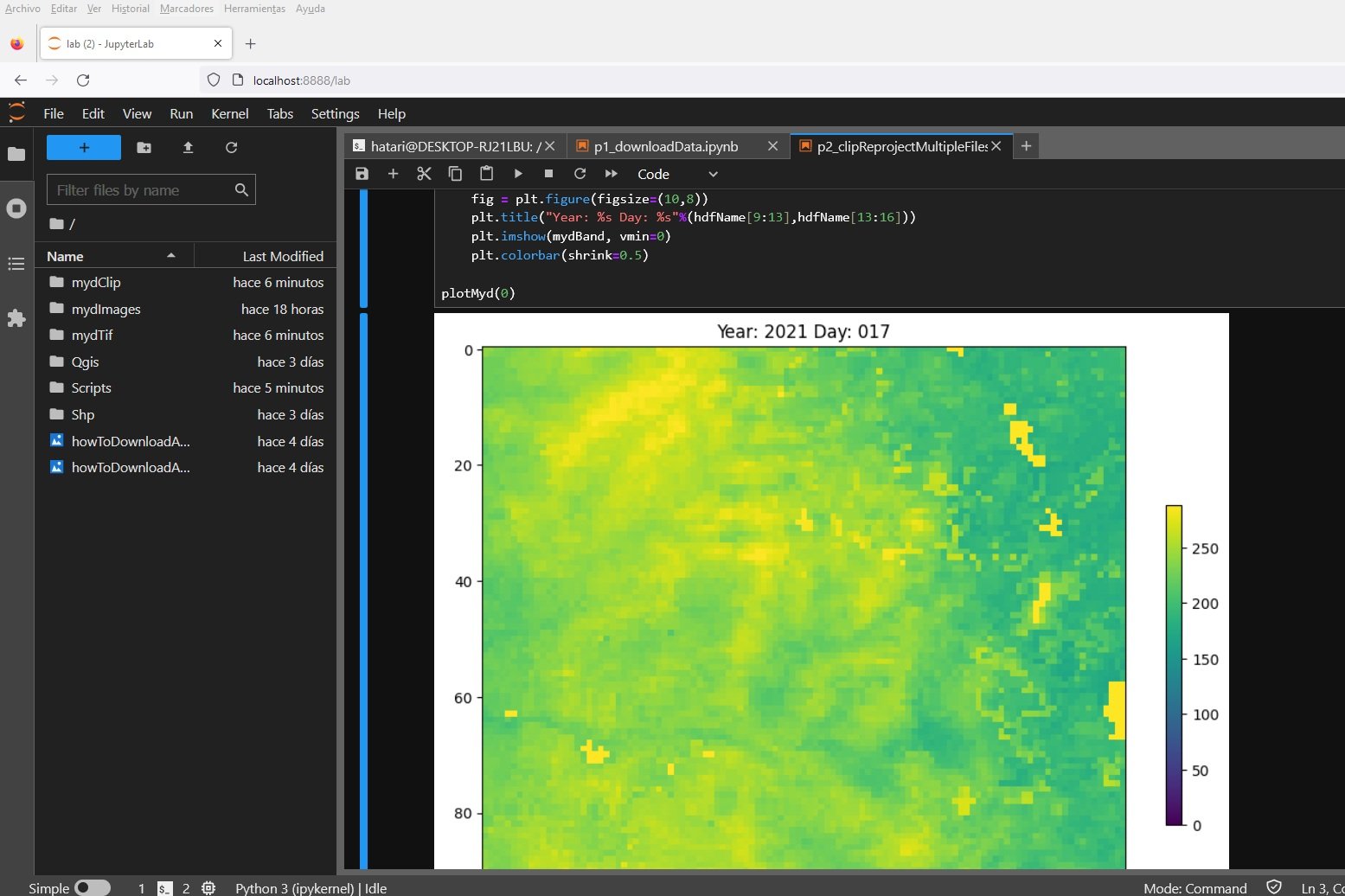
def plotMyd(hdfIndex):
    #open
    hdfName  = hdfList[hdfIndex][:-4]
    mydDS = gdal.Open(os.path.join('../mydClip',hdfName+'.tif'))
    mydBand = mydDS.GetRasterBand(1).ReadAsArray()
    #get rid of outliers
    mydBand[mydBand>maxValue] = maxValue
    fig = plt.figure(figsize=(10,8))
    plt.title("Year: %s Day: %s"%(hdfName[9:13],hdfName[13:16]))
    plt.imshow(mydBand, vmin=0)
    plt.colorbar(shrink=0.5)

plotMyd(0)

from ipywidgets import interact
import ipywidgets

slider = ipywidgets.IntSlider(
    value=0,
    min=0,
    max=len(hdfList) - 1,
    step=1,
    description='Hdf Index:',
    disabled=False,
    continuous_update=False,
    orientation='horizontal',
    readout=True,
    readout_format='d'
)

interact(plotMyd, hdfIndex=slider);

interactive(children=(IntSlider(value=0, continuous_update=False, description='Hdf Index:', max=9), Output()),…

Input data

Download the input files from this link.

Blog

How to reproject, clip and interactively plot HDFs with Python and GDAL - Tutorial

Animation

Tutorial

Python code

Input data

Hatari Labs

Our courses: