Satellite imagery brought us the capacity to see the land surface on recent years but we haven’t been so successful to understand land cover dynamics and the interaction with economical, sociological and political factors. Some deficiencies for this analysis were found on the use of GIS commercial software, but there are other limitations in the way we apply logical and mathematical processes to a set of satellite imagery. Working with geospatial data on Python gives us the capability to filter, calculate, clip, loop, and export raster or vector datasets with an efficient use of the computational power providing a bigger scope on data analysis.

This tutorial shows the complete procedure to create a land cover change raster from a comparison of generated vegetation index (NDVI) rasters by the use of Python and the Numpy and GDAL libraries. Contours of land cover change where generated with some tools of GDAL and Osgeo and an analysis of deforestation were done based on the output data and historical images from Google Earth.

Tutorial

Python code

This is the Python code for the tutorial:

Import requires libraries

This tutorial uses just Python core libraries, Scipy (Numpy, Matplotlib and others) and GDAL. For Windows users, the most effective way is to download the GDAL Wheel from https://www.lfd.uci.edu/~gohlke/pythonlibs/ and install through pip.

from osgeo import ogr, gdal, osr
import numpy as np
import os
import matplotlib.pyplot as plt

Setting up the input and output files

We declare the path for the raster bands and the output NDVI and land cover change rasters. The land cover change contour shape path is also defined.

#Input Raster and Vector Paths

#Image-2019
path_B5_2019="../Image20190203clip/LC08_L1TP_029047_20190203_20190206_01_T1_B5_clip.TIF"
path_B4_2019="../Image20190203clip/LC08_L1TP_029047_20190203_20190206_01_T1_B4_clip.TIF"

#Image-2014
path_B5_2014="../Image20140205clip/LC08_L1TP_029047_20140205_20170307_01_T1_B5_clip.TIF"
path_B4_2014="../Image20140205clip/LC08_L1TP_029047_20140205_20170307_01_T1_B4_clip.TIF"

#Output Files

#Output NDVI Rasters 
path_NDVI_2019 = '../Output/NDVI2019.tif'
path_NDVI_2014 = '../Output/NDVI2014.tif'
path_NDVIChange_19_14 = '../Output/NDVIChange_19_14.tif'

#NDVI Contours
contours_NDVIChange_19_14 = '../Output/NDVIChange_19_14.shp'

Open the Landsat image bands with GDAL

In this part we open the red (Band 4) and near infrared NIR (Band 5) with commands of the GDAL library and then we read the images as matrix arrays with float numbers of 32 bits.

#Open raster bands
B5_2019 = gdal.Open(path_B5_2019)
B4_2019 = gdal.Open(path_B4_2019)
B5_2014 = gdal.Open(path_B5_2014)
B4_2014 = gdal.Open(path_B4_2014)

#Read bands as matrix arrays
B52019_Data = B5_2019.GetRasterBand(1).ReadAsArray().astype(np.float32)
B42019_Data = B4_2019.GetRasterBand(1).ReadAsArray().astype(np.float32)
B52014_Data = B5_2014.GetRasterBand(1).ReadAsArray().astype(np.float32)
B42014_Data = B4_2014.GetRasterBand(1).ReadAsArray().astype(np.float32)

Compare matrix sizes and geotransformation parameters

The operation in between Landsat 8 bands depends that the resolution, size, src, and geotransformation parameters are the same for both images. In case these caracteristics do not coincide a warp, reproyection, scale or any other geospatial process would be necessary.

print(B5_2014.GetProjection()[:80])
print(B5_2019.GetProjection()[:80])
if B5_2014.GetProjection()[:80]==B5_2019.GetProjection()[:80]: print('SRC OK')

PROJCS["WGS 84 / UTM zone 13N",GEOGCS["WGS 84",DATUM["WGS_1984",SPHEROID["WGS 84
PROJCS["WGS 84 / UTM zone 13N",GEOGCS["WGS 84",DATUM["WGS_1984",SPHEROID["WGS 84
SRC OK

print(B52014_Data.shape)
print(B52019_Data.shape)
if B52014_Data.shape==B52019_Data.shape: print('Array Size OK')

(610, 597)
(610, 597)
Array Size OK

print(B5_2014.GetGeoTransform())
print(B5_2019.GetGeoTransform())
if B5_2014.GetGeoTransform()==B5_2019.GetGeoTransform(): print('Geotransformation OK')

(652500.0, 29.98324958123953, 0.0, 2166000.0, 0.0, -30.0)
(652500.0, 29.98324958123953, 0.0, 2166000.0, 0.0, -30.0)
Geotransformation OK

Get geotransformation parameters

Since we have compared that rasters bands have same array size and are in the same position we can get the some spatial parameters

geotransform = B5_2014.GetGeoTransform()

originX,pixelWidth,empty,finalY,empty2,pixelHeight=geotransform
cols =  B5_2014.RasterXSize
rows =  B5_2014.RasterYSize

projection = B5_2014.GetProjection()

finalX = originX + pixelWidth * cols
originY = finalY + pixelHeight * rows

Compute the NDVI and store them as a different file

We can compute the NDVI as a matrix algebra with some Numpy functions. The result can be exported as a raster using GDAL and the transformation parameters. In order to have a more effective and clear code we create a function to export rasters.

ndvi2014 = np.divide(B52014_Data - B42014_Data, B52014_Data+ B42014_Data,where=(B52014_Data - B42014_Data)!=0)
ndvi2014[ndvi2014 == 0] = -999

ndvi2019 = np.divide(B52019_Data - B42019_Data, B52019_Data+ B42019_Data,where=(B52019_Data - B42019_Data)!=0)
ndvi2019[ndvi2019 == 0] = -999

def saveRaster(dataset,datasetPath,cols,rows,projection):
    rasterSet = gdal.GetDriverByName('GTiff').Create(datasetPath, cols, rows,1,gdal.GDT_Float32)
    rasterSet.SetProjection(projection)
    rasterSet.SetGeoTransform(geotransform)
    rasterSet.GetRasterBand(1).WriteArray(dataset)
    rasterSet.GetRasterBand(1).SetNoDataValue(-999)
    rasterSet = None

saveRaster(ndvi2014,path_NDVI_2014,cols,rows,projection)

saveRaster(ndvi2019,path_NDVI_2019,cols,rows,projection)

Plot NDVI Images

We create a function to plot the resulting NDVI images with a colobar

extentArray = [originX,finalX,originY,finalY]
def plotNDVI(ndviImage,extentArray,vmin,cmap):
    ndvi = gdal.Open(ndviImage)
    ds2019 = ndvi.ReadAsArray()
    plt.figure(figsize=(20,15))
    im = plt.imshow(ds2019, vmin=vmin, cmap=cmap, extent=extentArray)#
    plt.colorbar(im, fraction=0.015)
    plt.xlabel('Este')
    plt.ylabel('Norte')
    plt.show()

plotNDVI(path_NDVI_2014,extentArray,0,'YlGn')

plotNDVI(path_NDVI_2019,extentArray,0,'YlGn')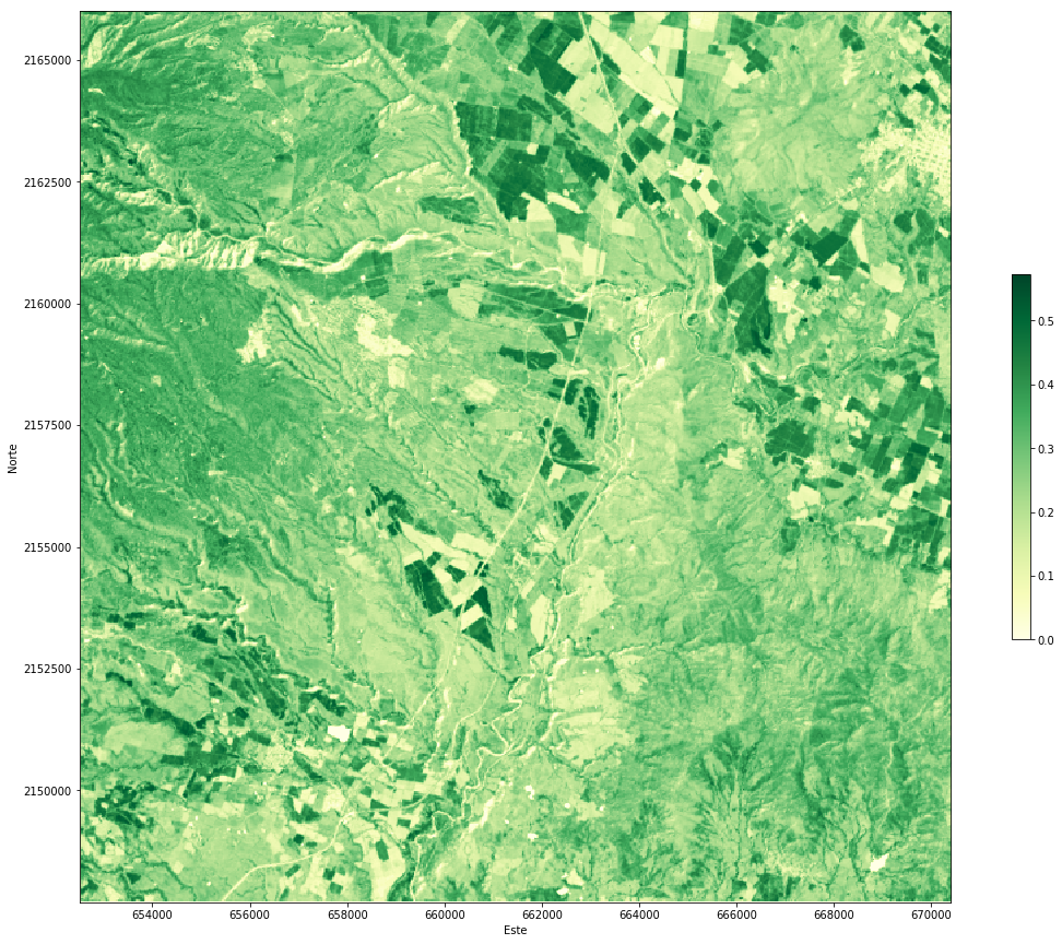

Create a land cover change image

We create a land cover change image based on the differences in NDVI from 2019 and 2014 imagery. The image will be stored as a separate file.

ndviChange = ndvi2019-ndvi2014
ndviChange = np.where((ndvi2014>-999) & (ndvi2019>-999),ndviChange,-999)
ndviChange

array([[-9.9900000e+02,  3.5470784e-02,  3.7951261e-02, ...,
         3.1590372e-02,  3.8002759e-02,  2.6692629e-02],
       [-9.9900000e+02,  3.7654012e-02,  5.8923483e-02, ...,
        -5.8691800e-03,  1.8922418e-02,  1.9506305e-02],
       [-9.9900000e+02,  3.2184020e-02,  3.7395060e-02, ...,
        -6.3773081e-02, -3.0675709e-02,  3.8942695e-02],
       ...,
       [-9.9900000e+02, -1.6597062e-02,  1.1402190e-02, ...,
         2.7218461e-03,  2.5526762e-02,  6.6639006e-02],
       [-9.9900000e+02,  5.9944689e-03, -4.0770471e-03, ...,
         5.7501763e-02,  4.6757758e-03,  8.4484324e-02],
       [-9.9900000e+02, -9.9900000e+02, -9.9900000e+02, ...,
        -9.9900000e+02, -9.9900000e+02, -9.9900000e+02]], dtype=float32)

saveRaster(ndviChange,path_NDVIChange_19_14,cols,rows,projection)

plotNDVI(path_NDVIChange_19_14,extentArray,-0.5,'Spectral')

Create Contourlines

Finally, the countour lines from the NDVI values are generated. This is done with tool from the GDAL library.

Dataset_ndvi = gdal.Open(path_NDVIChange_19_14)#path_NDVI_2014
ndvi_raster = Dataset_ndvi.GetRasterBand(1)

ogr_ds = ogr.GetDriverByName("ESRI Shapefile").CreateDataSource(contours_NDVIChange_19_14)

prj=Dataset_ndvi.GetProjectionRef()#GetProjection()

srs = osr.SpatialReference(wkt=prj)#
#srs.ImportFromProj4(prj)

contour_shp = ogr_ds.CreateLayer('contour', srs)
field_defn = ogr.FieldDefn("ID", ogr.OFTInteger)
contour_shp.CreateField(field_defn)
field_defn = ogr.FieldDefn("ndviChange", ogr.OFTReal)
contour_shp.CreateField(field_defn)
#Generate Contourlines
gdal.ContourGenerate(ndvi_raster, 0.1, 0, [], 1, -999, contour_shp, 0, 1)
ogr_ds = None