Having a reasonable spatial distribution of the water table with few observation points is a challenge because the water table can't be above the surface. We wanted to develop a method where the computer learns not only about the position but also the surface to calculate the water table.

This is an applied example of water level interpolation based on a machine learning algorithm in Python with Scikit Learn. The code covers all steps from data compilation, regression formulation, accuracy testing and raster generation.

Tutorial

Code

Working on the data compilation

# import packages to compile the data
import pandas as pd
import geopandas as gpd
import matplotlib.pyplot as plt
import numpy as np

### creation of a dataframe for the neural network
wakeLoc = pd.read_csv('../Csv/WakeCoNC_slugtest_Wells.csv', usecols=[2,3,4,6])
wakeLoc = wakeLoc.set_index('well_name_short')
wakeLoc.head()

	latitude_dd_nad1983	longitude_dd_nad1983	alt_mp_navd1988
well_name_short
CH-252	35.815336	-78.925508	336.48
WK-283	35.733056	-78.675556	359.70
WK-332	35.720833	-78.500556	192.26
WK-334	35.720833	-78.500556	190.95
WK-368	35.943000	-78.684000	410.06

#add a value of hydraulic conductiviy. We read the hydraulic conductivities from another file and create a mean
wakeK = pd.read_csv('../Csv/WakeCoNC_slugtest_Analyses.csv',usecols=[1,6,19])
meanValues = wakeK.groupby('well_name_short')[['wl_static_dbls']].mean()
meanValues[:5]

	wl_static_dbls
well_name_short
CH-252	41.2775
WK-283	29.9800
WK-332	16.8275
WK-334	15.2825
WK-368	121.0770

# apply the mean K to the original dataframe
wakeLoc['wlElev'] = -999.0
for index, row in wakeLoc.iterrows():
    wakeLoc.loc[index,'wlElev'] = wakeLoc.loc[index,'alt_mp_navd1988'] - meanValues.loc[index,'wl_static_dbls']

wakeLoc.to_csv('../Csv/wellDf.csv')
wakeLoc.tail()

	latitude_dd_nad1983	longitude_dd_nad1983	alt_mp_navd1988	wlElev
well_name_short
WK-433	35.585893	-78.678039	326.92	322.2050
WK-434	35.585893	-78.678039	328.43	301.4225
WK-435	35.642404	-78.825825	434.40	411.3175
WK-436	35.695548	-78.766925	435.93	412.4400
WK-437	35.695548	-78.766925	436.87	406.9200

Machine learning model construction

# import required packages
from sklearn.preprocessing import StandardScaler
from sklearn.neural_network import MLPRegressor
from sklearn.model_selection import train_test_split
from sklearn.metrics import r2_score, mean_squared_error
from sklearn.linear_model import LinearRegression

#define the two datasets
headValues = wakeLoc.iloc[:,3].values.reshape(-1,1) #because it is a single column
paramValues = wakeLoc.iloc[:,:3].values

# Define the scaler
headScaler = StandardScaler().fit(headValues)

# Scale the train set
headValuesScaled = headScaler.transform(headValues)
headValuesScaled[:5]

array([[-0.24772745],
       [ 0.27174055],
       [-2.05019526],
       [-2.04665865],
       [-0.34132725]])

# Check scaler over head values
print(headValuesScaled.mean(axis=0))
print(headValuesScaled.std(axis=0))

[-1.43675921e-16]
[1.]

# Define the scaler
paramScaler = StandardScaler().fit(paramValues)

# Scale the train set
paramValuesScaled = paramScaler.transform(paramValues)
paramValuesScaled[:5]

array([[ 0.29272505, -2.01170002, -0.03127219],
       [-0.35552737, -0.2333869 ,  0.29555826],
       [-0.45182133,  1.01166934, -2.06122429],
       [-0.45182133,  1.01166934, -2.07966305],
       [ 1.29853513, -0.29346549,  1.00439467]])

# Check scaler over param values
print(paramValuesScaled.mean(axis=0))
print(paramValuesScaled.std(axis=0))

[-4.61330320e-14 -7.14199941e-14  1.69798816e-16]
[1. 1. 1.]

# Split over Train and Test
headTrain, headTest, paramTrain, paramTest = train_test_split(headValuesScaled, paramValuesScaled, 
                                                              test_size=0.2, random_state=42)

# Regressor
regr = MLPRegressor(hidden_layer_sizes=(100,100,100),max_iter=50000).fit(paramTrain, headTrain)

c:\Users\saulm\anaconda3\Lib\site-packages\sklearn\neural_network\_multilayer_perceptron.py:1650: DataConversionWarning: A column-vector y was passed when a 1d array was expected. Please change the shape of y to (n_samples, ), for example using ravel().
  y = column_or_1d(y, warn=True)

# Get predicted values for test array
headPredict = regr.predict(paramTest)

# get the inverse for the test and predicted heads
headPredictedInversed = headScaler.inverse_transform(headPredict.reshape(-1,1))
headTestInversed = headScaler.inverse_transform(headTest.reshape(-1,1))

# Create single subplot
fig, ax = plt.subplots(figsize=(8, 6))

# Scatter plot
ax.scatter(headTestInversed, headPredictedInversed, alpha=0.7, label='Data')

# Regression line
x_line = np.linspace(headValues.min(), headValues.max(), 100).reshape(-1, 1)
ax.plot(x_line, x_line, color='red', linewidth=2, label='Indentity Line')

# Calculate metrics
r2 = r2_score(headTestInversed, headPredictedInversed)
rmse = np.sqrt(mean_squared_error(headTestInversed, headPredictedInversed))

# Add metrics as text
metrics_text = f'R² = {r2:.3f}\nRMSE = {rmse:.3f}'
ax.text(0.05, 0.95, metrics_text, transform=ax.transAxes, 
        verticalalignment='top', bbox=dict(boxstyle='round', facecolor='wheat'))

ax.set_xlabel('Heads Observed')
ax.set_ylabel('Heads Predicted')
ax.legend()
ax.grid(True, alpha=0.3)
plt.tight_layout()
plt.show()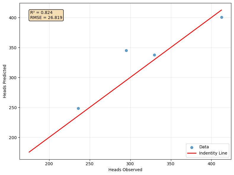

Create the interpolated raster

import rasterio
from rasterio.plot import show

#open dem and array
demFeet = rasterio.open('../Rst/areaDem_feet_NAD83_clip.tif')
demArray = demFeet.read(1)
demShape = demArray.shape
print(demShape)

(1094, 1440)

interpHeads = np.zeros(demShape)
paramTupleList = []

i = 0
for row in range(demShape[0]):
    for col in range(demShape[1]):
        x,y = demFeet.xy(row,col)
        #print(x,y)
        paramTuple = [y,x,demArray[row,col]] #lat, lon
        #print(x,y,demArray[row,col])
        #headPredict = v
        #paramTupleScaled = paramScaler.transform([paramTuple])
        paramTupleList.append(paramTuple)
     
        if i % 400000 == 0:
            print('processing %d cells, please be patient!'%i)
        i+=1

processing 0 cells, please be patient!
processing 400000 cells, please be patient!
processing 800000 cells, please be patient!
processing 1200000 cells, please be patient!

paramTupleScaledList = paramScaler.transform(paramTupleList)

demFeetMeta = demFeet.meta
demFeetMeta

{'driver': 'GTiff',
 'dtype': 'float32',
 'nodata': -3.4028234663852886e+38,
 'width': 1440,
 'height': 1094,
 'count': 1,
 'crs': CRS.from_wkt('GEOGCS["NAD83",DATUM["North_American_Datum_1983",SPHEROID["GRS 1980",6378137,298.257222101004,AUTHORITY["EPSG","7019"]],AUTHORITY["EPSG","6269"]],PRIMEM["Greenwich",0],UNIT["degree",0.0174532925199433,AUTHORITY["EPSG","9122"]],AXIS["Latitude",NORTH],AXIS["Longitude",EAST],AUTHORITY["EPSG","4269"]]'),
 'transform': Affine(0.000277776805555558, 0.0, -78.833190499,
        0.0, -0.0002777788464351009, 35.982082827)}

interpHeadsList = regr.predict(paramTupleScaledList)
interpHeadsListInversed = headScaler.inverse_transform(interpHeadsList.reshape(-1,1))
interpHeadsListInversed

array([[345.69730345],
       [348.84354167],
       [347.86908141],
       ...,
       [205.89600829],
       [205.91801105],
       [208.86160631]])

interpHeadsArray = interpHeadsListInversed.reshape(demShape)
plt.imshow(interpHeadsArray)

<matplotlib.image.AxesImage at 0x231937267b0>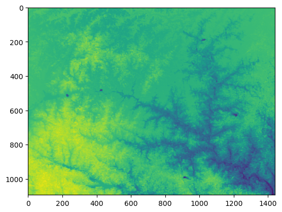

interpRaster = rasterio.open('../Rst/interpRaster.tif','w',**demFeetMeta)

interpRaster.write(interpHeadsArray,1)

interpRaster.close()

Input data

You can download the input data from this link:

owncloud.hatarilabs.com/s/pyv9obJnyObR52m

Password: Hatarilabs

Blog

Machine learning based interpolation for regional water table w. Python and Scikit Learn - Tutorial

Tutorial

Code

Working on the data compilation

Machine learning model construction

Create the interpolated raster

Input data

Hatari Labs

Our courses:

Blog

Tutorial

Code

Working on the data compilation

Machine learning model construction

Create the interpolated raster

Input data

Hatari Labs

Our courses:

Follow Us

Join us on social media for the latest webinars, tutorials and courses.