

Regional example of seawater intrusion modeling with MODFLOW6 and mf6Voronoi - Tutorial
/
This is an applied example of seawater intrusion modeling using MODFLOW6 and the BUY package. The model is fully geospatial and works with ESRI Shapefiles and rasters (*.tif) as inputs. The model grid is based on Voronoi meshes generated with the Python package mf6Voronoi. Since there are so many concepts involved in the conceptualization of a variable density groundwater flow simulation with MODFLOW6 and Flopy, these cases use a code template from mf6Voronoi that simplifies the model construction and simulation. The applied case also gives us the chance to discuss the main parts of model setup.
Tutorial
Code
from mf6Voronoi.utils import listTemplates, copyTemplate#listTemplates()copyTemplate('generateVoronoi','wkRegional')copyTemplate('seawaterIntrusion','wkRegional')copyTemplate('vtkGeneration','wkRegional')Mesh generation
Part 1 : Voronoi mesh generation
import warnings ## Org
warnings.filterwarnings('ignore') ## Org
import os, sys ## Org
import geopandas as gpd ## Org
from mf6Voronoi.geoVoronoi import createVoronoi ## Org
from mf6Voronoi.meshProperties import meshShape ## Org
from mf6Voronoi.utils import initiateOutputFolder, getVoronoiAsShp ## Org
#Create mesh object specifying the coarse mesh and the multiplier
vorMesh = createVoronoi(meshName='regionalSeawaterIntrusion',maxRef = 500, multiplier=1.5) ## Org
#Open limit layers and refinement definition layers
vorMesh.addLimit('basin','../shp/modelAoi.shp') ## Org
vorMesh.addLayer('ref','../shp/modelRef.shp',100) ## Org
vorMesh.addLayer('stream1','../hatariUtils1/river_basin.shp',150) ## Org
vorMesh.addLayer('stream2','../hatariUtils2/river_basin.shp',150) ## Org
vorMesh.addLayer('well','../shp/pumpingWells.shp',50) ## Org
vorMesh.addLayer('obs','../shp/obsPoints.shp',50) ## Org
vorMesh.addLayer('sea','../shp/seaGhb.shp',400) ## Org#Generate point pair array
vorMesh.generateOrgDistVertices() ## Org
#Generate the point cloud and voronoi
vorMesh.createPointCloud() ## Org
vorMesh.generateVoronoi() ## Org
mf6Voronoi will have a web version in 2028
Follow us: |
 |
 |
 |
 |
 |
 |
/--------Layer ref discretization-------/
Progressive cell size list: [100, 250.0, 475.0] m.

/--------Layer stream1 discretization-------/
Progressive cell size list: [150, 375.0] m.

/--------Layer stream2 discretization-------/
Progressive cell size list: [150, 375.0] m.

/--------Layer well discretization-------/
Progressive cell size list: [50, 125.0, 237.5, 406.25] m.

/--------Layer obs discretization-------/
Progressive cell size list: [50, 125.0, 237.5, 406.25] m.

/--------Layer sea discretization-------/
Progressive cell size list: [400] m.

/----Sumary of points for voronoi meshing----/
Distributed points from layers: 6
Points from layer buffers: 6065
Points from max refinement areas: 1085
Points from min refinement areas: 616
Total points inside the limit: 8837
/--------------------------------------------/

Time required for point generation: 1.27 seconds


/----Generation of the voronoi mesh----/

Time required for voronoi generation: 0.73 seconds
#Uncomment the next two cells if you have strong differences on discretization or you have encounter an FORTRAN error while running MODFLOW6vorMesh.checkVoronoiQuality(threshold=0.01)/----Performing quality verification of voronoi mesh----/
Short side on polygon: 8817 with length = 0.00834
Short side on polygon: 8817 with length = 0.00834
Short side on polygon: 8817 with length = 0.00053
Short side on polygon: 8817 with length = 0.00053
Short side on polygon: 8817 with length = 0.00722
Short side on polygon: 8817 with length = 0.00722vorMesh.fixVoronoiShortSides()
vorMesh.generateVoronoi()
vorMesh.checkVoronoiQuality(threshold=0.01)/----Generation of the voronoi mesh----/
Time required for voronoi generation: 0.71 seconds
/----Performing quality verification of voronoi mesh----/
Your mesh has no edges shorter than your threshold#Export generated voronoi mesh
initiateOutputFolder('../output') ## Org
getVoronoiAsShp(vorMesh.modelDis, shapePath='../output/'+vorMesh.modelDis['meshName']+'.shp') ## OrgThe output folder ../output exists and has been cleared
/----Generation of the voronoi shapefile----/
Time required for voronoi shapefile: 1.54 seconds# Show the resulting voronoi mesh
#open the mesh file
mesh=gpd.read_file('../output/'+vorMesh.modelDis['meshName']+'.shp') ## Org
#plot the mesh
mesh.plot(figsize=(35,25), fc='crimson', alpha=0.3, ec='teal') ## Org<Axes: >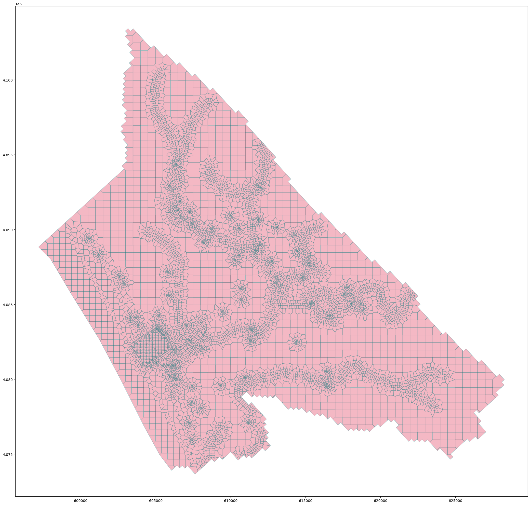
Part 2 generate disv properties
# open the mesh file
mesh=meshShape('../output/'+vorMesh.modelDis['meshName']+'.shp') ## Org
# get the list of vertices and cell2d data
gridprops=mesh.get_gridprops_disv() ## OrgCreating a unique list of vertices [[x1,y1],[x2,y2],...]
100%|██████████| 8821/8821 [00:00<00:00, 20737.11it/s]
Extracting cell2d data and grid index
100%|██████████| 8821/8821 [00:02<00:00, 3556.41it/s]#create folder
initiateOutputFolder('../json') ## Org
#export disv
mesh.save_properties('../json/disvDict.json') ## OrgThe output folder ../json exists and has been clearedMultilayer and transient model
Part 2a: generate disv properties
import sys, json, os ## Org
import rasterio, flopy ## Org
import numpy as np ## Org
import matplotlib.pyplot as plt ## Org
import geopandas as gpd ## Org
from mf6Voronoi.meshProperties import meshShape ## Org
from shapely.geometry import MultiLineString ## Org
from mf6Voronoi.tools.cellWork import getLayCellElevTupleFromRaster, getLayCellElevTupleFromElev, getLayCellElevTupleFromObs
# open the json file
with open('../json/disvDict.json') as file: ## Org
gridProps = json.load(file) ## Orgcell2d = gridProps['cell2d'] #cellid, cell centroid xy, vertex number and vertex id list
vertices = gridProps['vertices'] #vertex id and xy coordinates
ncpl = gridProps['ncpl'] #number of cells per layer
nvert = gridProps['nvert'] #number of verts
centroids=gridProps['centroids'] #cell centroids xyPart 2b: Model construction and simulation
#Extract dem values for each centroid of the voronois
from shapely.geometry import Point

src = rasterio.open('../rst/modelDem.tif')  ## Org
seaDf = gpd.read_file('../shp/seaBeach.shp') #<==== updated

elevation = [] #initialize list

for centroid in centroids: #fix values of raster inside the sea polygon
    centPoint = Point(centroid) #get geometry of the cell centroid

    if centPoint.within(seaDf.iloc[0].geometry): #if it is inside the sea
        elevation.append(0)
    else:
        elevation += [x[0].item() for x in src.sample([centroid])] #assing raster value
elevation[1000:1005]
[0, 292, 0, 55, 49]nlay = 8 ## Org
mtop=np.array(elevation) #[elev[0] for i,elev in enumerate(elevation)]) ## Org
zbot=np.zeros((nlay,ncpl)) ## Org
AcuifInf_Bottom = -150# <==== update
zbot[0,] = AcuifInf_Bottom + (0.875 * (mtop - AcuifInf_Bottom)) ## Org
zbot[1,] = AcuifInf_Bottom + (0.75 * (mtop - AcuifInf_Bottom)) ## Org
zbot[2,] = AcuifInf_Bottom + (0.625 * (mtop - AcuifInf_Bottom)) ## Org
zbot[3,] = AcuifInf_Bottom + (0.5 * (mtop - AcuifInf_Bottom)) ## Org
zbot[4,] = AcuifInf_Bottom + (0.375 * (mtop - AcuifInf_Bottom)) ## Org
zbot[5,] = AcuifInf_Bottom + (0.25 * (mtop - AcuifInf_Bottom)) ## Org
zbot[6,] = AcuifInf_Bottom + (0.125 * (mtop - AcuifInf_Bottom)) ## Org
zbot[7,] = AcuifInf_Bottom ## OrgCreate simulation and model
# create simulation
simName = 'mf6Sim' ## Org
modelName = 'mf6Model' ## Org
modelWs = '../modelFiles' ## Org
sim = flopy.mf6.MFSimulation(sim_name=simName, version='mf6', ## Org
                             exe_name='../bin/mf6.exe', ## Org
                             continue_=True,
                             sim_ws=modelWs) ## Org
# create tdis package
tdis_rc = [(86400.0*365*50, 1, 1.0)] + [(86400*365*30, 1, 1.0)] ## 30 years, 15 years, 15 years
#tdis_rc = [(86400.0*365*50, 1, 1.0)] + [(86400*365*30, 1, 1.0) for level in range(2)] ## 30 years, 15 years, 15 years
print(tdis_rc[:3]) ## Org
tdis = flopy.mf6.ModflowTdis(sim, pname='tdis', time_units='SECONDS', ## Org
perioddata=tdis_rc, ## Org
nper=2) ## Org[(1576800000.0, 1, 1.0), (946080000, 1, 1.0)]# create gwf model
gwf = flopy.mf6.ModflowGwf(sim, ## Org
modelname=modelName, ## Org
save_flows=True, ## Org
newtonoptions="NEWTON UNDER_RELAXATION") ## Org# create iterative model solution and register the gwf model with it
imsGwf = flopy.mf6.ModflowIms(sim, ## Org
pname='ims_gwf',
complexity='COMPLEX', ## Org
outer_maximum=150, ## Org
inner_maximum=50, ## Org
outer_dvclose=0.1, ## Org
inner_dvclose=0.0001, ## Org
backtracking_number=20, ## Org
linear_acceleration='BICGSTAB') ## Org
sim.register_ims_package(imsGwf,[modelName]) ## Org# disv
disv = flopy.mf6.ModflowGwfdisv(gwf, nlay=nlay, ncpl=ncpl, ## Org
top=mtop, botm=zbot, ## Org
nvert=nvert, vertices=vertices, ## Org
cell2d=cell2d) ## Orgdisv.top.plot(figsize=(12,8), alpha=0.8) ## Org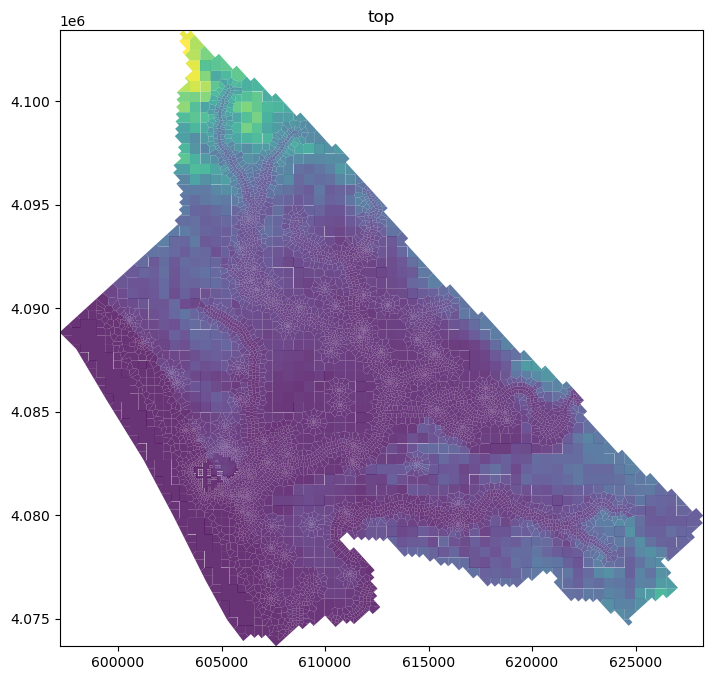
crossSection = gpd.read_file('../shp/crossSection.shp') ## Org
sectionLine =list(crossSection.iloc[0].geometry.coords) ## Org

fig, ax = plt.subplots(figsize=(12,8)) ## Org
modelxsect = flopy.plot.PlotCrossSection(model=gwf, line={'Line': sectionLine}) ## Org
linecollection = modelxsect.plot_grid(lw=0.5) ## Org
ax.set_ylim(-150,100)
ax.grid() ## Org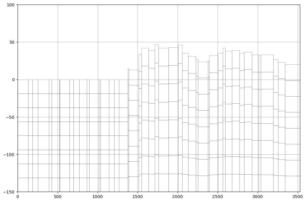
# initial conditions
ic = flopy.mf6.ModflowGwfic(gwf, strt=np.stack([mtop for i in range(nlay)])) ## Org
Kx =[4E-3 for x in range(3)] + [1E-3 for x in range(3)] + [4E-4 for x in range(2)] ## <=== updated
icelltype = [1 for x in range(5)] + [0 for x in range(nlay - 5)] ## Org
# node property flow
npf = flopy.mf6.ModflowGwfnpf(gwf, ## Org
save_specific_discharge=True, ## Org
icelltype=icelltype, ## Org
k=Kx, ## Org
k33=Kx) ## <== updated# define storage and transient stress periods
sto = flopy.mf6.ModflowGwfsto(gwf, ## Org
iconvert=1, ## Org
steady_state={ ## Org
0:True, ## Org
},
transient={
1:True, ## Org
2:True, ## Org
},
ss=1e-06,
sy=0.001,
) ## OrgWorking with rechage, evapotranspiration
rchr = 0.2/365/86400 ## Org
rch = flopy.mf6.ModflowGwfrcha(gwf, recharge=rchr) ## Org
evtr = 1.2/365/86400 ## Org
evt = flopy.mf6.ModflowGwfevta(gwf,ievt=1,surface=mtop,rate=evtr,depth=1.0) ## Org
Definition of the intersect object
For the manipulation of spatial data to determine hydraulic parameters or boundary conditions
# Define intersection object
interIx = flopy.utils.gridintersect.GridIntersect(gwf.modelgrid) ## Org
#general boundary condition
ghbSpd = {} ## # <===== Inserted
ghbSpd[0] = [] ## # <===== Inserted
# #regional flow
# layCellTupleList, cellElevList = getLayCellElevTupleFromRaster(gwf,
# interIx,
# '../rst/waterTable.tif',
# '../shp/regGhb.shp') ## # <===== Inserted
# for index, layCellTuple in enumerate(layCellTupleList): ## Org
# ghbSpd[0].append([layCellTuple,cellElevList[index],0.01, 0, 'regflow']) # <===== Inserted
layCellTupleList = getLayCellElevTupleFromElev(gwf,
interIx,
0,
'../shp/seaGhb.shp',)
for layCellTuple in layCellTupleList:
ghbSpd[0].append([layCellTuple, 0, 0.20, 0, 'sea'])You have inserted a fixed elevationghb = flopy.mf6.ModflowGwfghb(gwf, stress_period_data=ghbSpd, auxiliary=['CONCENTRATION'], boundnames=True) ## <==== modified
# Observation package for Drain
obsDict = { # <===== Inserted
"{}.ghb.obs.csv".format(modelName): [ # <===== Inserted
("regflow", "ghb", "regionalFlow"), # <===== Inserted
("sea", "ghb", "sea") # <===== Inserted
] # <===== Inserted
} # <===== Inserted
# Attach observation package to DRN package
ghb.obs.initialize( # <===== Inserted
filename=gwf.name+".ghb.obs", # <===== Inserted
digits=10, # <===== Inserted
print_input=True, # <===== Inserted
continuous=obsDict # <===== Inserted
) # <===== Inserted#define buy package
buyModName = 'modelBuy'
Csalt = 35.
Cfresh = 0.
densesalt = 1025.
densefresh = 1000.
denseslp = (densesalt - densefresh) / (Csalt - Cfresh)
pd = [(0, denseslp, 0., buyModName, 'CONCENTRATION')]
buy = flopy.mf6.ModflowGwfbuy(gwf, denseref=1000., nrhospecies=1,packagedata=pd)#ghb plot
ghb.plot(mflay=0, kper=0) # <===== Inserted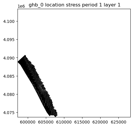
from copy import copy
#well bc

wellSpd = {} ## # <===== Inserted
wellSpd[0] = [] ## # <===== Inserted
wellSpd[1] = []

#regional flow
# from raster
# layCellTupleList, cellElevList = getLayCellElevTupleFromRaster(gwf,
#                                                                interIx,
#                                                                '../rst/modelDemMinus45.tif',
#                                                                '../shp/wellsStage1.shp') ## # <===== Inserted

# for index, layCellTuple in enumerate(layCellTupleList): ## Org
#     wellSpd[1].append([layCellTuple,-0.01,'wellsStage1']) # <===== Inserted

# from elevation
layCellTupleList = getLayCellElevTupleFromElev(gwf,
                                               interIx,
                                               -20,
                                               '../shp/pumpingWells.shp',)
for layCellTuple in layCellTupleList:
    wellSpd[1].append([layCellTuple, -0.01, 'wellsStage1'])

wellSpd[1][:10]
You have inserted a fixed elevation
[[(3, 2857), -0.01, 'wellsStage1'],
[(3, 2712), -0.01, 'wellsStage1'],
[(3, 2959), -0.01, 'wellsStage1'],
[(2, 3392), -0.01, 'wellsStage1'],
[(2, 4731), -0.01, 'wellsStage1'],
[(2, 3561), -0.01, 'wellsStage1'],
[(2, 5838), -0.01, 'wellsStage1'],
[(2, 4952), -0.01, 'wellsStage1'],
[(2, 4255), -0.01, 'wellsStage1'],
[(2, 3988), -0.01, 'wellsStage1']]wel = flopy.mf6.ModflowGwfwel(gwf, stress_period_data=wellSpd, boundnames=True) ## <==== modified
# Observation package for Drain
obsDict = { # <===== Inserted
"{}.wel.obs.csv".format(modelName): [ # <===== Inserted
("wellsStage1", "wel", "wellsStage1") # <===== Inserted
] # <===== Inserted
} # <===== Inserted
# Attach observation package to DRN package
wel.obs.initialize( # <===== Inserted
filename=gwf.name+".wel.obs", # <===== Inserted
digits=10, # <===== Inserted
print_input=True, # <===== Inserted
continuous=obsDict # <===== Inserted
) # <===== InsertedrefBounds = gpd.read_file('../shp/modelRef.shp').total_bounds
#ghb plot
fig, ax = plt.subplots()
#
mV = flopy.plot.PlotMapView(gwf)
mV.plot_bc('WEL', kper=1, ax=ax, plotAll=True)
mV.plot_bc('GHB', kper=1, ax=ax)
mV.plot_grid(alpha=0.5, lw=0.2)
ax.set_xlim(refBounds[0]-1000,refBounds[2]+1000)
ax.set_ylim(refBounds[1]-1000,refBounds[3]+1000)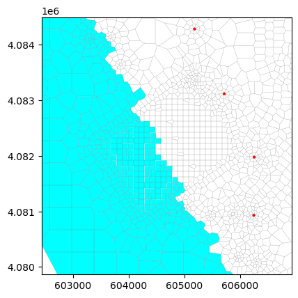
#open the river shapefile
rivers =gpd.read_file('../hatariUtils1/river_basin.shp') ## Org

list_rivers=[] ## Org
for i in range(rivers.shape[0]): ## Org
    list_rivers.append(rivers['geometry'].loc[i]) ## Org

riverMls = MultiLineString(lines=list_rivers) ## Org

#intersec rivers with our grid
riverCells=interIx.intersect(riverMls).cellids ## Org
riverCells[:10] ## Org
array([895, 920, 1084, 1115, 1143, 1158, 1183, 1190, 1191, 1192],
dtype=object)#river package
riverSpd = {} ## Org
riverSpd[0] = [] ## Org
for cell in riverCells: ## Org
riverSpd[0].append([(0,cell),mtop[cell],0.01]) ## Org#open the river shapefile
rivers =gpd.read_file('../hatariUtils2/river_basin.shp') ## Org
list_rivers=[] ## Org
for i in range(rivers.shape[0]): ## Org
list_rivers.append(rivers['geometry'].loc[i]) ## Org
riverMls = MultiLineString(lines=list_rivers) ## Org
#intersec rivers with our grid
riverCells=interIx.intersect(riverMls).cellids ## Org
for cell in riverCells: ## Org
riverSpd[0].append([(0,cell),mtop[cell],0.01]) ## Orgriv = flopy.mf6.ModflowGwfdrn(gwf, stress_period_data=riverSpd) ## Org
#river plot
riv.plot(mflay=0) ## Org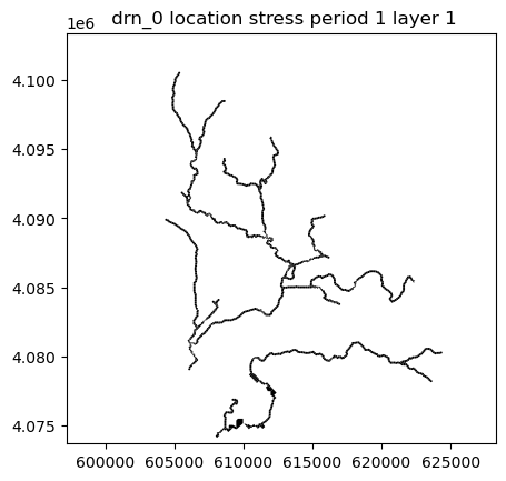
Define transport model
#create transport package
gwt = flopy.mf6.ModflowGwt(sim, modelname=buyModName)

#register solver for transport model
imsGwt = flopy.mf6.ModflowIms(sim,
                              pname='ims_gwt',
                              #print_option='SUMMARY', ## Org
                              outer_dvclose=2e-4, ## Org
                              inner_dvclose=3e-4, ## Org
                              linear_acceleration='BICGSTAB') ## Org
sim.register_ims_package(imsGwt,[gwt.name])

#define spatial discretization
gwtDisv = flopy.mf6.ModflowGwtdisv(gwt, nlay=disv.nlay.data,
                                   ncpl=disv.ncpl.data,
                                   nvert=disv.nvert.data,
                                   top=disv.top.data,
                                   botm=disv.botm.data,
                                   vertices=disv.vertices.array.tolist(),
                                   cell2d=disv.cell2d.array.tolist(),
                                  )
## Org
sim.register_ims_package(imsGwf,[modelName])
#sim.write_simulation()#define starting concentrations
strtConc = np.zeros((disv.nlay.data, disv.ncpl.data), dtype=np.float32)
ghbList = ghb.stress_period_data.array[0].tolist()
ghbList[-5:][((0, 3827), 0, 0.2, 0, 'sea'),
((0, 3840), 0, 0.2, 0, 'sea'),
((0, 3841), 0, 0.2, 0, 'sea'),
((0, 3862), 0, 0.2, 0, 'sea'),
((0, 3894), 0, 0.2, 0, 'sea')]for ghbItem in ghbList:
if ghbItem[4] == 'sea':
strtConc[:,ghbItem[0][1]] = 35 #apply for all layers below the ghb
gwtIc = flopy.mf6.ModflowGwtic(gwt, strt=strtConc)# create plot of initial concentratios
fig = plt.figure(figsize=(12, 12))
ax = fig.add_subplot(1, 1, 1, aspect = 'equal')
mapview = flopy.plot.PlotMapView(model=gwf,layer = 1)
plot_array = mapview.plot_array(strtConc,masked_values=[-1e+30], cmap=plt.cm.summer)
plt.colorbar(plot_array, shrink=0.75,orientation='horizontal', pad=0.08, aspect=50)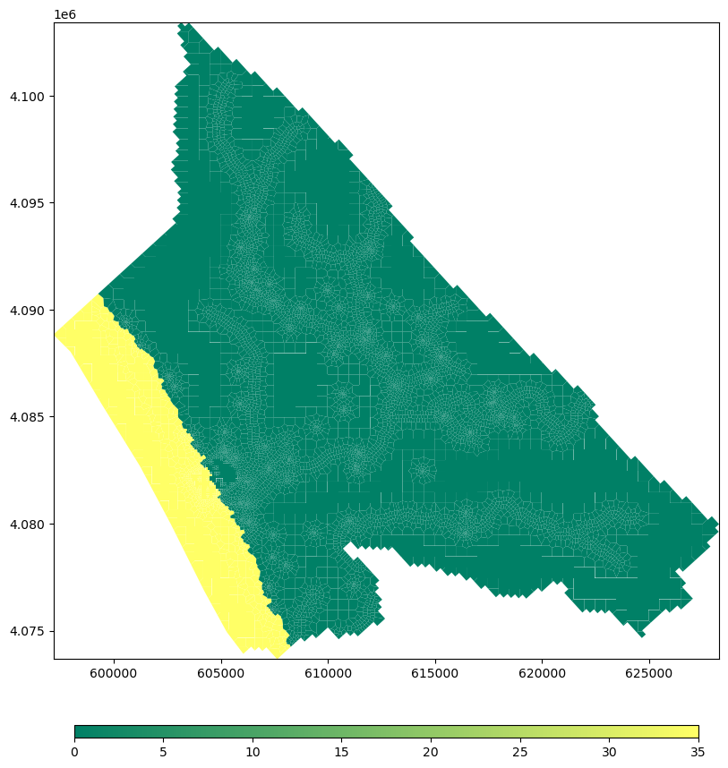
#define advection
adv = flopy.mf6.ModflowGwtadv(gwt, scheme='UPSTREAM')
#define dispersion
dsp = flopy.mf6.ModflowGwtdsp(gwt,alh=10,ath1=10)
#define mobile storage and transfer
porosity = 0.30
sto = flopy.mf6.ModflowGwtmst(gwt, porosity=porosity)
#define sink and source package
sourcerecarray = ['GHB_0','AUX','CONCENTRATION']
ssm = flopy.mf6.ModflowGwtssm(gwt, sources=sourcerecarray)
#define constant concentration package
cncSp = []
for row in ghb.stress_period_data.array[0]:
if row['boundname'] == 'sea':
cncSp.append([row[0],35])
cncSpd = {0:cncSp,1:cncSp}
cnc = flopy.mf6.ModflowGwtcnc(gwt,stress_period_data=cncSpd)
# cnc.plot(mflay=0, lw=0.1, figsize=(12,12))#working with observation points
obsList = []
nameList, obsLayCellList = getLayCellElevTupleFromObs(gwf, ## Org
interIx, ## Org
'../shp/obsPoints.shp', ## Org
'Name', ## Org
'Elev') ## Org
for obsName, obsLayCell in zip(nameList, obsLayCellList): ## Org
obsList.append((obsName,'concentration',obsLayCell[0]+1,obsLayCell[1]+1)) ## Org
obs = flopy.mf6.ModflowUtlobs( ## Org
gwt,
filename=gwt.name+'.obs', ## Org
digits=10, ## Org
print_input=True, ## Org
continuous={gwt.name+'.obs.csv': obsList} ## Org
)Working for cell 436
Well screen elev of -20.00 found at layer 2
Working for cell 132
Well screen elev of -20.00 found at layer 2
Working for cell 132
Well screen elev of -20.00 found at layer 2
Working for cell 132
Well screen elev of -20.00 found at layer 2
Working for cell 206
Well screen elev of -20.00 found at layer 1
Working for cell 206
Well screen elev of -20.00 found at layer 1
Working for cell 206
Well screen elev of -20.00 found at layer 1
Working for cell 370
Well screen elev of -20.00 found at layer 3
Working for cell 370
Well screen elev of -20.00 found at layer 3
Working for cell 370
Well screen elev of -20.00 found at layer 3
Working for cell 370
Well screen elev of -20.00 found at layer 3
Working for cell 699
Well screen elev of -20.00 found at layer 1
Working for cell 641
Well screen elev of -20.00 found at layer 2
Working for cell 551
Well screen elev of -20.00 found at layer 1
Working for cell 551
Well screen elev of -20.00 found at layer 1
Working for cell 2025
Well screen elev of -20.00 found at layer 1
Working for cell 2025
Well screen elev of -20.00 found at layer 1
Working for cell 1711
Well screen elev of -20.00 found at layer 1
Working for cell 1346
Well screen elev of -20.00 found at layer 1
Working for cell 1346
Well screen elev of -20.00 found at layer 1
Working for cell 2171
Well screen elev of -20.00 found at layer 1
Working for cell 2554
Well screen elev of -20.00 found at layer 1
Working for cell 3361
Well screen elev of -20.00 found at layer 1
Working for cell 3521
Well screen elev of -20.00 found at layer 1
Working for cell 1485
Well screen elev of -20.00 found at layer 2
Working for cell 3541
Well screen elev of -20.00 found at layer 1Set the output control and exchange / run model
#oc for flow
head_filerecord = f"{gwf.name}.hds" ## Org
budget_filerecord = f"{gwf.name}.cbc" ## Org
oc = flopy.mf6.ModflowGwfoc(gwf, ## Org
                            head_filerecord=head_filerecord, ## Org
                            budget_filerecord = budget_filerecord, ## Org
                            saverecord=[("HEAD", "LAST"),("BUDGET","LAST")]) ## Org

#oc for transport
oc = flopy.mf6.ModflowGwtoc(gwt,
                            concentration_filerecord=buyModName+'.ucn',
                            saverecord=[('CONCENTRATION', 'ALL')])

#define model flow and transport exchange
name = 'modelExchange'
gwfgwt = flopy.mf6.ModflowGwfgwt(sim, exgtype='GWF6-GWT6',
                                 exgmnamea=gwf.name, exgmnameb=buyModName,
                                 filename='{}.gwfgwt'.format(name))
# Run the simulation
sim.write_simulation() ## Orgwriting simulation...
writing simulation name file...
writing simulation tdis package...
writing solution package ims_gwt...
writing solution package ims_gwf...
writing package modelExchange.gwfgwt...
writing model mf6Model...
writing model name file...
writing package disv...
writing package ic...
writing package npf...
writing package sto...
writing package rcha_0...
writing package evta_0...
writing package ghb_0...
INFORMATION: maxbound in ('gwf6', 'ghb', 'dimensions') changed to 792 based on size of stress_period_data
writing package obs_0...
writing package buy...
writing package wel_0...
INFORMATION: maxbound in ('gwf6', 'wel', 'dimensions') changed to 69 based on size of stress_period_data
writing package obs_1...
writing package drn_0...
INFORMATION: maxbound in ('gwf6', 'drn', 'dimensions') changed to 1068 based on size of stress_period_data
writing package oc...
writing model modelBuy...
writing model name file...
writing package disv...
writing package ic...
writing package adv...
writing package dsp...
writing package mst...
writing package ssm...
writing package cnc_0...
INFORMATION: maxbound in ('gwt6', 'cnc', 'dimensions') changed to 792 based on size of stress_period_data
writing package obs_0...
writing package oc...success, buff = sim.run_simulation() ## OrgFloPy is using the following executable to run the model: ..\bin\mf6.exe
MODFLOW 6
U.S. GEOLOGICAL SURVEY MODULAR HYDROLOGIC MODEL
VERSION 6.6.0 12/20/2024
MODFLOW 6 compiled Dec 31 2024 17:10:16 with Intel(R) Fortran Intel(R) 64
Compiler Classic for applications running on Intel(R) 64, Version 2021.7.0
Build 20220726_000000
This software has been approved for release by the U.S. Geological
Survey (USGS). Although the software has been subjected to rigorous
review, the USGS reserves the right to update the software as needed
pursuant to further analysis and review. No warranty, expressed or
implied, is made by the USGS or the U.S. Government as to the
functionality of the software and related material nor shall the
fact of release constitute any such warranty. Furthermore, the
software is released on condition that neither the USGS nor the U.S.
Government shall be held liable for any damages resulting from its
authorized or unauthorized use. Also refer to the USGS Water
Resources Software User Rights Notice for complete use, copyright,
and distribution information.
MODFLOW runs in SEQUENTIAL mode
Run start date and time (yyyy/mm/dd hh:mm:ss): 2025/12/12 12:02:58
Writing simulation list file: mfsim.lst
Using Simulation name file: mfsim.nam
Solving: Stress period: 1 Time step: 1
Solving: Stress period: 2 Time step: 1
Run end date and time (yyyy/mm/dd hh:mm:ss): 2025/12/12 12:04:20
Elapsed run time: 1 Minutes, 22.849 Seconds
Normal termination of simulation.Model output visualization
headObj = gwf.output.head() ## Org
headObj.get_kstpkper() ## Org
[(np.int32(0), np.int32(0)), (np.int32(0), np.int32(1))]kper = 0 ## Org
lay = 0 ## Orgheads = headObj.get_data(kstpkper=(0,kper))
#heads[lay,0,:5]
#heads = headObj.get_data(kstpkper=(0,0))
#np.save('npy/headCalibInitial', heads)### Plot the heads for a defined layer and boundary conditions
fig = plt.figure(figsize=(12,8)) ## Org
ax = fig.add_subplot(1, 1, 1, aspect='equal') ## Org
modelmap = flopy.plot.PlotMapView(model=gwf) ## Org
####
levels = np.linspace(heads[heads>-1e+30].min(),heads[heads>-1e+30].max(),num=50) ## Org
contour = modelmap.contour_array(heads[lay],ax=ax,levels=levels,cmap='PuBu')
ax.clabel(contour) ## Org
quadmesh = modelmap.plot_bc('GHB') ## Org
cellhead = modelmap.plot_array(heads[lay],ax=ax, cmap='Blues', alpha=0.8)
#linecollection = modelmap.plot_grid(linewidth=0.3, alpha=0.5, color='cyan', ax=ax) ## Org
plt.colorbar(cellhead, shrink=0.75) ## Org
plt.show() ## Org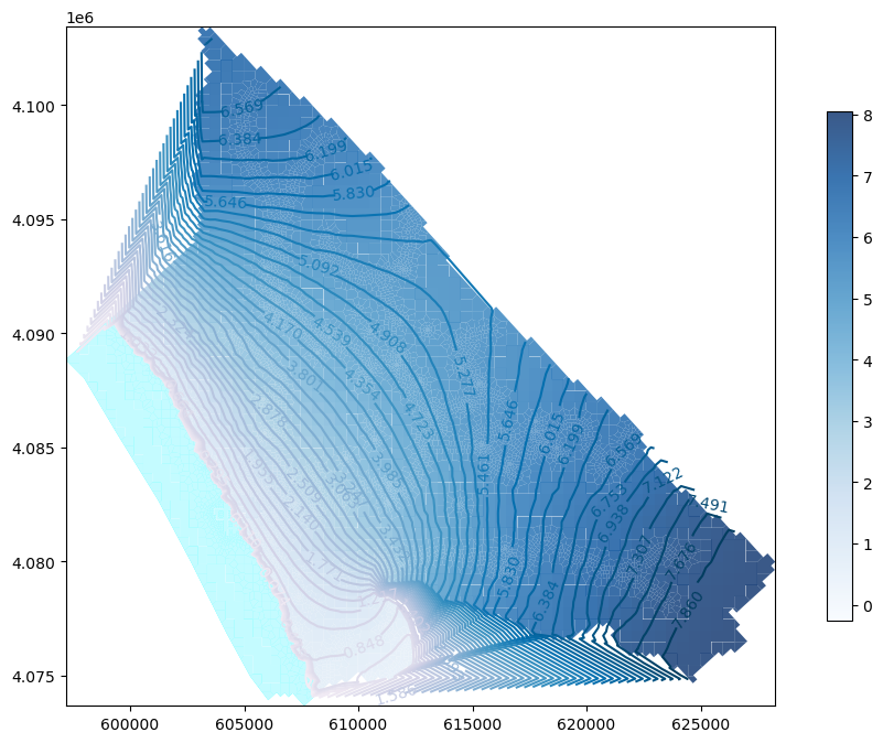
crossSection = gpd.read_file('../shp/crossSection.shp')
sectionLine =list(crossSection.iloc[0].geometry.coords)

waterTable = flopy.utils.postprocessing.get_water_table(heads)

fig, ax = plt.subplots(figsize=(12,8))
xsect = flopy.plot.PlotCrossSection(model=gwf, line={'Line': sectionLine})
lc = xsect.plot_grid(lw=0.5)
xsect.plot_array(heads, alpha=0.5)
xsect.plot_surface(waterTable)
xsect.plot_bc('ghb', kper=kper, facecolor='none', edgecolor='teal')
plt.show()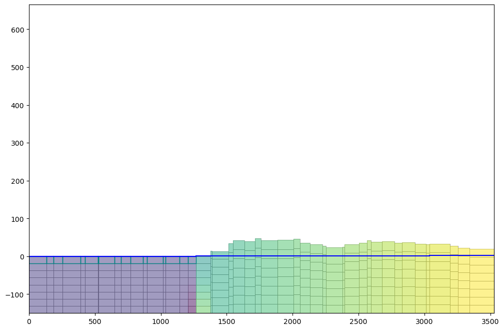
Explore the concentration results
concObj = gwt.output.concentration() ## Org
concObj.get_kstpkper() ## Org
[(np.int32(0), np.int32(0)), (np.int32(0), np.int32(1))]#define time series and stress period to plot
ts = (0,1)
#get concentrations for the time step
tempConc = concObj.get_data(kstpkper=ts)### Review the flow model
fig = plt.figure(figsize=(12, 12))
ax = fig.add_subplot(1, 1, 1, aspect = 'equal')
mapview = flopy.plot.PlotMapView(model=gwf,layer = 4)
plot_array = mapview.plot_array(tempConc,masked_values=[-1e+30], cmap=plt.cm.summer)
plt.colorbar(plot_array, shrink=0.75,orientation='horizontal', pad=0.08, aspect=50)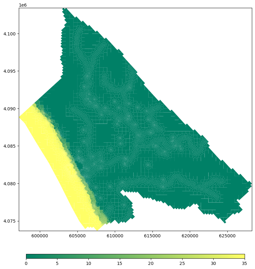
### Zoom to intrusion
# fig = plt.figure(figsize=(12, 12))
# ax = fig.add_subplot(1, 1, 1, aspect = 'equal')
# mapview = flopy.plot.PlotMapView(model=gwf,layer = 4)

# plot_array = mapview.plot_array(tempConc,masked_values=[-1e+30], cmap=plt.cm.summer)
# plt.colorbar(plot_array, shrink=0.75,orientation='horizontal', pad=0.08, aspect=50)
# ax.set_xlim(200000,206000)
# ax.set_ylim(8798000,8803000)
#plot heads on line
tempHead = headObj.get_data(kstpkper=ts)
fig, ax = plt.subplots(figsize=(18,6))
crossSection = gpd.read_file('../shp/crossSection.shp')
sectionLine =list(crossSection.iloc[0].geometry.coords)
crossview = flopy.plot.PlotCrossSection(model=gwf, line={"line": sectionLine})
crossview.plot_grid(alpha=0.25)
strtArray = crossview.plot_array(tempConc, masked_values=[1e30], cmap=plt.cm.summer)
cb = plt.colorbar(strtArray, shrink=0.5)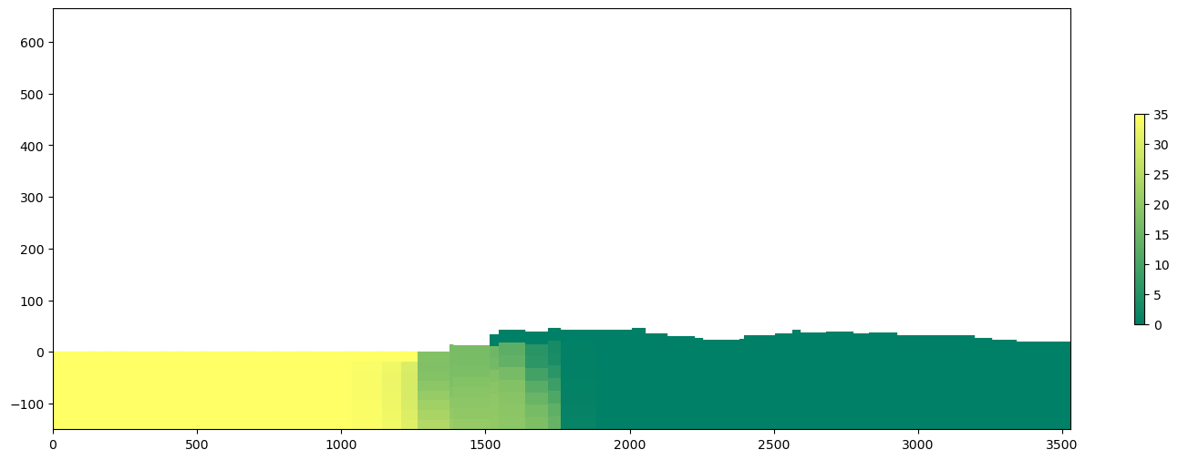
Input data
You can download the input data from this link:
https://owncloud.hatarilabs.com/s/Soro1nFyRBJdoD0
Password to download files: Hatarilabs.


