Effective stress theory was developed by Terzaghi in the 1920s. Based on our modeling experience we wanted to calculate the effective stress based on the results from a MODFLOW groundwater model. Finally, after 6 years from the first thought about it we came with a full deduction of the effective stress calculation based on the model geometry and an applied example for the effective stress calculation on a hillslope groundwater flow model.

The example model was developed in Modflow-Nwt and Model Muse, whereas the effective stress determination was done with scripts in Python and Hataripy (our fork of Flopy). The scripts can also generate 3D objects as VTK files of the model results, geometry and stresses that can be visualized in Paraview.

Effective stress calculation

Tutorial

Coding

This in the Python for the effective stress calculation and geometry generation:

import hataripy
import numpy as np
import matplotlib.pyplot as plt

hataripy is installed in C:\Users\saulm\anaconda3\lib\site-packages\hataripy

Open model and heads

#define model name, path, executables
modelWs = '../Model/'
modName = 'HillslopeModel_v1d_mf2005'
nwtPath = '../Exe/MODFLOW-NWT_64.exe'

#load model
mf = hataripy.modflow.Modflow.load(modName+'.nam', model_ws=modelWs, verbose=False,
                               check=False, exe_name=nwtPath)

# get a list of the model packages
mf.get_package_list()

['DIS', 'BAS6', 'OC', 'NWT', 'UPW', 'GHB', 'DRN', 'RCH']

# open binary head file
headFile = hataripy.utils.binaryfile.HeadFile(modelWs + modName + '.bhd')
headFile.get_times()

[1.0]

# get array of heads
headArray = headFile.get_data(totim=1.0)
headArray.shape

(20, 57, 46)

#plot surface topography
plt.imshow(mf.modelgrid.top)

<matplotlib.image.AxesImage at 0x28f1f09ac70>

Effective stress calculation

# calculate water table from heads
waterTableArray = np.zeros([headArray.shape[1],headArray.shape[2]])
for row in range(headArray.shape[1]):
    for col in range(headArray.shape[2]):
        heads=headArray[:,row,col]
        if heads[heads>-1e+20].size > 0:
            waterTableArray[row,col]=round(heads[heads>-1e+20][0],3)
        else:
            waterTableArray[row,col]=-1e+20

#plot water table
plt.imshow(waterTableArray)

<matplotlib.image.AxesImage at 0x28f1f819190>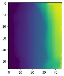

# H1 determination
H1 = np.zeros(headArray.shape)

for lay in range(headArray.shape[0]):
    H1[lay] = np.where((mf.modelgrid.top>waterTableArray)&(waterTableArray>mf.modelgrid.botm[lay]),
                       mf.modelgrid.top-waterTableArray,0)

# H2 determination
H2 = np.zeros(headArray.shape)

for lay in range(headArray.shape[0]):
    H2[lay] = np.where((mf.modelgrid.top>waterTableArray)&(waterTableArray>mf.modelgrid.zcellcenters[lay]),
                      waterTableArray-mf.modelgrid.zcellcenters[lay],0)

# HCell determination
HCell = np.zeros(headArray.shape)

for lay in range(headArray.shape[0]):
    oneCellHead = headArray[lay] - mf.modelgrid.zcellcenters[lay]
    HCell[lay] = np.where(oneCellHead>0, oneCellHead, 0)

rhoUnsat = 15 # in kN/m3 as reference value 
rhoSat = 19 # in kN/m3 as reference value 
rhoWater = 9.8 # in kN/m3

effectiveStress = rhoUnsat*H1 + rhoSat*H2 - rhoWater*HCell

#plot effective stresses for lay 1
plt.imshow(effectiveStress[0])

<matplotlib.image.AxesImage at 0x28f1f867ac0>

#plot effective stresses for row 25
plt.imshow(effectiveStress[:,25,:])

Working on the VTK

# get information about the drain cells
drnCells = mf.drn.stress_period_data[0]

# get information about the ghb cells
ghbCells = mf.ghb.stress_period_data[0]

# add the arrays to the vtkObject
vtkObject = hataripy.export.vtk.Vtk3D(mf,'../vtuFiles/',verbose=True)
vtkObject.add_array('head',headArray)
vtkObject.add_array('drn',drnCells)
vtkObject.add_array('ghb',ghbCells)

# add the effective stress array
vtkObject.add_array('effectivestress',effectiveStress)

# Create the VTKs for model output, boundary conditions and water table
vtkObject.modelMesh('modelMesh.vtu',smooth=True,cellvalues=['head','effectivestress'])
vtkObject.modelMesh('modelDrn.vtu',smooth=True,cellvalues=['drn'],boundary='drn',avoidpoint=True)
vtkObject.modelMesh('modelGhb.vtu',smooth=True,cellvalues=['ghb'],boundary='ghb',avoidpoint=True)
vtkObject.waterTable('waterTable.vtu',smooth=True)

Writing vtk file: modelMesh.vtu
Number of point is 419520, Number of cells is 52440

Writing vtk file: modelDrn.vtu
Number of point is 2072, Number of cells is 259

Writing vtk file: modelGhb.vtu
Number of point is 11064, Number of cells is 1383

Writing vtk file: waterTable.vtu
Number of point is 10488, Number of cells is 2622