Groundwater modeling of a pumping test over a confined aquifer with MODFLOW-6 and FloPy - Tutorial
/We have done an applied groundwater model for a pumping test on a confined aquifer. The wellsite is located on the Clairborne aquifer (Georgia, USA) and has two observations on different layers besides the well itself. The aquifer test has two periods of pumping and recovery that last 3 days each one and the numerical model was constructed with MODFLOW-6 based on a Python script with the FloPy package. Comparison among observed and simulated wells were done with plots in Matplotlib.
Tutorial
#import required packages
import os, sys, copy
import matplotlib as mpl
import matplotlib.pyplot as plt
import numpy as np
import pandas as pd
import flopy
#model meta information
sim_name = "pumpingTest"
length_units = "meters"
time_units = "days"
ws = "../Model/"#spatial distribution
top = 49.07 # Top of the model
botmDict = {}
botmDict['Lay1'] = {'topElev':49.07,'botElev':32.31,'lyn':2}
botmDict['Lay2'] = {'topElev':32.31,'botElev':-25.29,'lyn':3}
botmDict['Lay3'] = {'topElev':-25.29,'botElev':-57.60,'lyn':3}
botmDict['Lay4'] = {'topElev':-57.60,'botElev':-164.29,'lyn':3}
botmList = []
repeatList = []
for key, value in botmDict.items():
botmList.append(np.linspace(value['topElev'],value['botElev'],value['lyn']+1)[1:])
repeatList.append(value['lyn'])
botm = np.hstack(botmList)
print(botm)
print(repeatList)
# Number of layers, cols, rows
nlay = botm.shape[0]
ncol = 121
nrow = 121
delr = delc = [4 for i in range(20)] + [2 for i in range(20)] + [0.5 for i in range(41)] + \
[2 for i in range(20)] + [4 for i in range(20)][ 40.69 32.31 13.11 -6.09 -25.29
-36.06 -46.83 -57.6 -93.16333333 -128.72666667
-164.29 ]
[2, 3, 3, 3]# Starting head
strt = np.hstack([np.array(43.43),np.linspace(43.43,36.033,3)])
strt = np.repeat(strt,[2, 3, 3, 3])
strtarray([43.43 , 43.43 , 43.43 , 43.43 , 43.43 , 39.7315, 39.7315,
39.7315, 36.033 , 36.033 , 36.033 ])icelltype = np.repeat(np.array([1, 0, 0, 0]),repeatList) # Cell conversion type
k11 = np.repeat(np.array([1e-3, 1e-5, 1e-6, 3e-5]),repeatList) # Horizontal hydraulic conductivity
k33 = np.array(k11)/10 #[1e-4, 1e-5, 1e-7, 1e-5] # Vertical hydraulic conductivity
ss = 1.0e-4 # Specific storage
sy = 0.02 # Specific yield (unitless)#3days pumping + 3days recovery = 6 days => each hour = 72 stress periods + 1 steady state
nper = 7 #1s, 3 days pumping, 3 days recovery => 73#temporal discretization
perlen = [1.0]+ [86400 for i in range(6)]
nstp = [1,8,3,3,8,3,3]
tsmult = [1.0, 2, 2, 1, 2, 1, 1]
tdis_ds = list(zip(perlen, nstp, tsmult))
tdis_ds[:5][(1.0, 1, 1.0), (86400, 8, 2), (86400, 3, 2), (86400, 3, 1), (86400, 8, 2)]#solver parameters
nouter = 50
ninner = 100
hclose = 1e-9
rclose = 1e-6#build model
sim_ws = os.path.join(ws, sim_name)
sim_ws'../Model/pumpingTest'#initalize simulation, temporal discretization and solver
sim = flopy.mf6.MFSimulation(
sim_name=sim_name,
sim_ws=sim_ws,
exe_name="../Bin/mf6.exe",
)
flopy.mf6.ModflowTdis(sim, nper=nper, perioddata=tdis_ds, time_units=time_units)
flopy.mf6.ModflowIms(
sim,
outer_maximum=nouter,
outer_dvclose=hclose,
inner_maximum=ninner,
inner_dvclose=hclose,
rcloserecord=f"{rclose} strict",
)<flopy.mf6.data.mfstructure.MFDataItemStructure object at 0x0000022C81878950>
package_name = ims_-1
filename = pumpingTest.ims
package_type = ims
model_or_simulation_package = simulation
simulation_name = pumpingTest
Block nonlinear
--------------------
outer_dvclose
{internal}
(1e-09)
outer_maximum
{internal}
(50)
Block linear
--------------------
inner_maximum
{internal}
(100)
inner_dvclose
{internal}
(1e-09)
rcloserecord
{internal}
(rec.array([('inner_rclose', 1.e-06, 'strict')],
dtype=[('inner_rclose_label', 'O'), ('inner_rclose', '<f8'), ('rclose_option', 'O')]))#groundwater model, spatial discretization, flow package and initial conditions
gwf = flopy.mf6.ModflowGwf(sim, modelname=sim_name, save_flows=True)
flopy.mf6.ModflowGwfdis(
gwf,
length_units=length_units,
nlay=nlay,
nrow=nrow,
ncol=ncol,
delr=delr,
delc=delc,
top=top,
botm=botm,
)
flopy.mf6.ModflowGwfnpf(
gwf,
cvoptions="perched",
perched=True,
icelltype=icelltype,
k=k11,
k33=k33,
save_specific_discharge=True,
)
flopy.mf6.ModflowGwfic(gwf, strt=strt)
flopy.mf6.ModflowGwfsto(
gwf,
iconvert=1,
ss=ss,
sy=sy,
steady_state={0: True},
transient={1: True},
)package_name = sto
filename = pumpingTest.sto
package_type = sto
model_or_simulation_package = model
model_name = pumpingTest
Block griddata
--------------------
iconvert
{constant 1}
ss
{constant 0.0001}
sy
{constant 0.02}
Block period
--------------------
steady-state
{internal}
(True)
transient
{internal}
(True)#model grid plot
fig = plt.figure(figsize=(10, 10))
ax = fig.add_subplot(1, 1, 1, aspect='equal')
gwf.modelgrid.plot(lw=0.5)
ax.set_xlim(50,200)
ax.set_ylim(50,200)(50.0, 200.0)
#modelgrid cross section
fig = plt.figure(figsize=(10, 8))
ax = fig.add_subplot(1, 1, 1, aspect='equal')
crossSection = flopy.plot.PlotCrossSection(model=gwf, line={'row': 10})
crossSection.plot_grid(ax=ax)
<matplotlib.collections.PatchCollection at 0x22c81c81d50>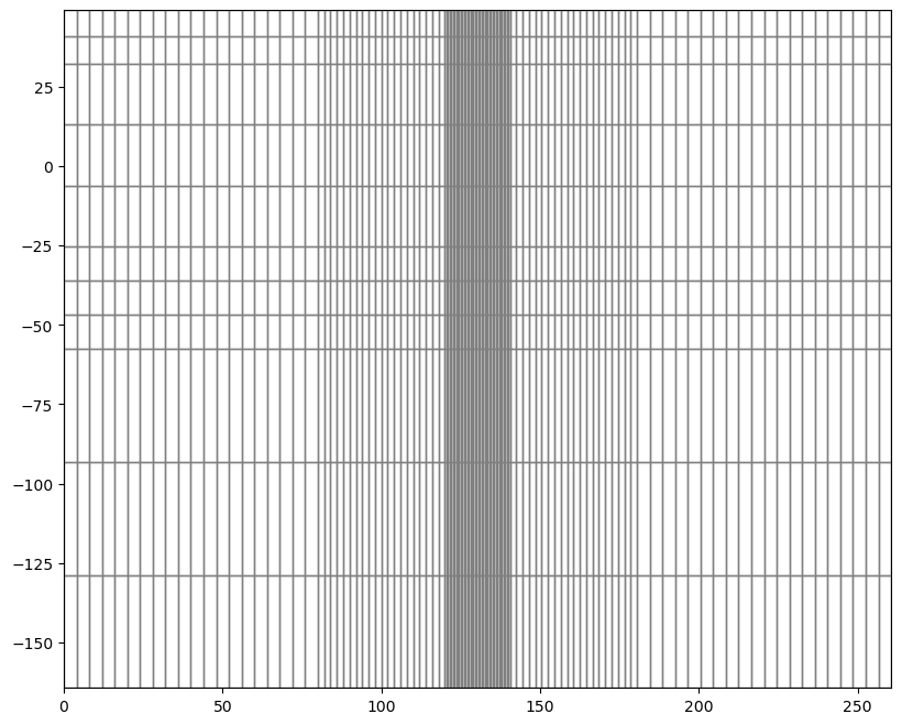
#general head boundary for regional flow
ghbSpd = []
for lay in range(nlay):
    for col in range(ncol):
        ghbSpd += [[lay,col,0,strt[lay],0.001]] #first col
        ghbSpd += [[lay,col,ncol-1,strt[lay],0.001]] #last col
        ghbSpd += [[lay,0,col,strt[lay],0.001]] #first row
        ghbSpd += [[lay,ncol-1,col,strt[lay],0.001]] #last row
ghbSpd = {0:ghbSpd}

ghb = flopy.mf6.ModflowGwfghb(
            gwf,
            stress_period_data=ghbSpd,
        )
#pumping well
welSpd = {}
welSpd[0] = [9,61,72,0]
welSpd[1] = [9,61,72,-0.03648] #579 gpm for 72hours
welSpd[4] = [9,61,72,0] #well deactivation
flopy.mf6.ModflowGwfwel(gwf, stress_period_data=welSpd)package_name = wel_0
filename = pumpingTest.wel
package_type = wel
model_or_simulation_package = model
model_name = pumpingTest
Block period
--------------------
stress_period_data
{internal}
(rec.array([((9, 61, 72), 0.)],
dtype=[('cellid', 'O'), ('q', '<f8')]))#output control
head_filerecord = f"{sim_name}.hds"
budget_filerecord = f"{sim_name}.cbc"
flopy.mf6.ModflowGwfoc(
gwf,
head_filerecord=head_filerecord,
budget_filerecord=budget_filerecord,
saverecord=[("HEAD", "ALL"), ("BUDGET", "ALL")],
)package_name = oc
filename = pumpingTest.oc
package_type = oc
model_or_simulation_package = model
model_name = pumpingTest
Block options
--------------------
budget_filerecord
{internal}
(rec.array([('pumpingTest.cbc',)],
dtype=[('budgetfile', 'O')]))
head_filerecord
{internal}
(rec.array([('pumpingTest.hds',)],
dtype=[('headfile', 'O')]))
Block period
--------------------
saverecord
{internal}
(rec.array([('HEAD', 'ALL', None), ('BUDGET', 'ALL', None)],
dtype=[('rtype', 'O'), ('ocsetting', 'O'), ('ocsetting_data', 'O')]))
printrecord
None#observation points
obsdict = {}
obslist = [["11J025", "head", (9, 61, 50)],
["11J029", "head", (9, 61, 72)],
["11J030", "head", (3, 61, 61)]]
obsdict[f"{sim_name}.obs.head.csv"] = obslist
obs = flopy.mf6.ModflowUtlobs(gwf, print_input=False, continuous=obsdict)sim.write_simulation()writing simulation...
writing simulation name file...
writing simulation tdis package...
writing solution package ims_-1...
writing model pumpingTest...
writing model name file...
writing package dis...
writing package npf...
writing package ic...
writing package sto...
writing package ghb_0...
INFORMATION: maxbound in ('gwf6', 'ghb', 'dimensions') changed to 5324 based on size of stress_period_data
writing package wel_0...
INFORMATION: maxbound in ('gwf6', 'wel', 'dimensions') changed to 1 based on size of stress_period_data
writing package oc...
writing package obs_0...sim.check()Checking model "pumpingTest"...
pumpingTest MODEL DATA VALIDATION SUMMARY:
No errors or warnings encountered.
Checks that passed:
npf package: zero or negative horizontal hydraulic conductivity values
npf package: vertical hydraulic conductivity values below checker threshold of 1e-11
npf package: vertical hydraulic conductivity values above checker threshold of 100000.0
npf package: horizontal hydraulic conductivity values below checker threshold of 1e-11
npf package: horizontal hydraulic conductivity values above checker threshold of 100000.0
sto package: zero or negative specific storage values
sto package: specific storage values below checker threshold of 1e-06
sto package: specific storage values above checker threshold of 0.01
sto package: zero or negative specific yield values
sto package: specific yield values below checker threshold of 0.01
sto package: specific yield values above checker threshold of 0.5
ghb_0 package: BC indices valid
ghb_0 package: not a number (Nan) entries
ghb_0 package: BC in inactive cells
wel_0 package: BC indices valid
wel_0 package: not a number (Nan) entries
wel_0 package: BC in inactive cells
Checking for missing simulation packages...
[<flopy.utils.check.mf6check at 0x22c81cc0c90>]sim.run_simulation()FloPy is using the following executable to run the model: ..\..\Bin\mf6.exe
MODFLOW 6
U.S. GEOLOGICAL SURVEY MODULAR HYDROLOGIC MODEL
VERSION 6.4.1 Release 12/09/2022
MODFLOW 6 compiled Dec 10 2022 05:57:01 with Intel(R) Fortran Intel(R) 64
Compiler Classic for applications running on Intel(R) 64, Version 2021.7.0
Build 20220726_000000
This software has been approved for release by the U.S. Geological
Survey (USGS). Although the software has been subjected to rigorous
review, the USGS reserves the right to update the software as needed
pursuant to further analysis and review. No warranty, expressed or
implied, is made by the USGS or the U.S. Government as to the
functionality of the software and related material nor shall the
fact of release constitute any such warranty. Furthermore, the
software is released on condition that neither the USGS nor the U.S.
Government shall be held liable for any damages resulting from its
authorized or unauthorized use. Also refer to the USGS Water
Resources Software User Rights Notice for complete use, copyright,
and distribution information.
Run start date and time (yyyy/mm/dd hh:mm:ss): 2023/12/22 9:57:43
Writing simulation list file: mfsim.lst
Using Simulation name file: mfsim.nam
Solving: Stress period: 1 Time step: 1
Solving: Stress period: 2 Time step: 1
Solving: Stress period: 2 Time step: 2
Solving: Stress period: 2 Time step: 3
Solving: Stress period: 2 Time step: 4
Solving: Stress period: 2 Time step: 5
Solving: Stress period: 2 Time step: 6
Solving: Stress period: 2 Time step: 7
Solving: Stress period: 2 Time step: 8
Solving: Stress period: 3 Time step: 1
Solving: Stress period: 3 Time step: 2
Solving: Stress period: 3 Time step: 3
Solving: Stress period: 4 Time step: 1
Solving: Stress period: 4 Time step: 2
Solving: Stress period: 4 Time step: 3
Solving: Stress period: 5 Time step: 1
Solving: Stress period: 5 Time step: 2
Solving: Stress period: 5 Time step: 3
Solving: Stress period: 5 Time step: 4
Solving: Stress period: 5 Time step: 5
Solving: Stress period: 5 Time step: 6
Solving: Stress period: 5 Time step: 7
Solving: Stress period: 5 Time step: 8
Solving: Stress period: 6 Time step: 1
Solving: Stress period: 6 Time step: 2
Solving: Stress period: 6 Time step: 3
Solving: Stress period: 7 Time step: 1
Solving: Stress period: 7 Time step: 2
Solving: Stress period: 7 Time step: 3
Run end date and time (yyyy/mm/dd hh:mm:ss): 2023/12/22 9:58:56
Elapsed run time: 1 Minutes, 13.479 Seconds
Normal termination of simulation.
(True, [])
For head comparison
import pandas as pd#open the simulation heads
simHead = pd.read_csv('../Model/pumpingTest/pumpingTest.obs.head.csv',index_col=0)
simHead.head()| 11J025 | 11J029 | 11J030 | |
|---|---|---|---|
| time | |||
| 1.000000 | 36.052406 | 36.052393 | 43.289912 |
| 339.823529 | 34.055220 | 10.303132 | 43.289912 |
| 1017.470588 | 31.723297 | 6.605409 | 43.289912 |
| 2372.764706 | 29.662453 | 4.251582 | 43.289912 |
| 5083.352941 | 27.897002 | 2.393536 | 43.289912 |
#open the observation points
w11J025 = pd.read_csv('../Txt/wtElev_11J025_timeDelta', index_col=0)
w11J029 = pd.read_csv('../Txt/wtElev_11J029_timeDelta', index_col=0)
w11J030 = pd.read_csv('../Txt/wtElev_11J030_timeDelta', index_col=0)
#head comparison
import matplotlib.pyplot as plt
fig, ax = plt.subplots()
w11J025.plot(ax=ax)
simHead['11J025'].plot(ax=ax, style='*-')
plt.legend()<matplotlib.legend.Legend at 0x1c1a4358990>