Modern times records lots of data, and computational software can deal with high amount of data, but we certainly haven’t been able to store efficiently data. We publish reports, we create tables and maps, but we are more focused on giving opinion and evaluations rather than in preserving the data that someone else can review and incorporate to its own study or reanalyze and provide a complete different evaluation.

Vector spatial data is a type of data, that are points, lines and polygons with related information. In order to give a complete value of this spatial data, it has to be stored in special OGC standards and ESRI Shapefiles, GeoJson, Klm, NetCDF, in commercial / open source databases, on web repositories. However, most times, the disorder and limited resources of public / private institutions makes the data available just on reports in digital version (as PDF) and even as paper based reports.

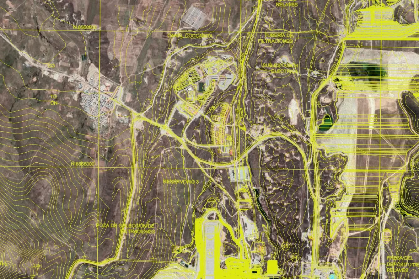
In order to use the spatial data provided on a report we need procedures to extract the data on effective way. The amount of tools and techniques are quite advanced, and requires several open source software for specific procedures. We have done a complete tutorial with all the step required to extract the vector spatial data of a map reported as PDF into a ESRI shapefile. For this tutorial we have used Inkscape for the conversion of the PDF to DXF, QGIS to extract some information of the DXF, Python and Geopandas on a Jupyter Lab session for spatial translation and scaling.

Tutorial

Python code

This is the python code used on the tutorial:

%matplotlib inline
import matplotlib.pyplot as plt
import geopandas as gpd

#open the DXF file
plano = gpd.read_file('../Pdf/Plano_Ccamacmayo.dxf')
plano.plot(figsize=(20,40))

partialTranslation=plano.translate(261.75756,-149.51527,0)
partialTranslation.plot(figsize=(20,40))
plt.grid()

scale = 4500/509.931 #1/193.11
geometryScaled = partialTranslation.scale(scale,scale,1, origin=(0,0,0)) #-261.75756,149.41021-261.66994,
geometryTranslated = geometryScaled.translate(249000, 8350500,0) #30.24975, 99.84579
geometryTranslated.plot(figsize=(20,40))
plt.grid()

#apply the new geometry to the geopandas dataframe and apply the EPSG cpde
plano = gpd.GeoDataFrame(plano, geometry=geometryTranslated)
plano.crs = {'init':'epsg:24789'}
plano.plot(figsize=(20,40))

#filter only the line elements
planoLines = plano[plano.geometry.type=='LineString']
#export the spatial as shapefile
planoLines.to_file('../Shps/Dxf_Total.shp')