On a normal groundwater modeling workflow the hydraulic parameters, observed data and boundary conditions are preprocessed on a GIS software as QGIS, and then imported on a compatible format (vector or raster) into the modeling software. However, Model Muse has a set of different tools to process point, and tabular data into model parameters increasing the speed in the model construction and simulation. This tutorial show the procedure to interpolate hydraulic conductivity from a table into Modflow from a different set of interpolation methods in Model Muse.

Interpolation methods

Model Muse can perform interpolate only 2D data sets. There are eight interpolation methods available in Model Muse:

Nearest Point: determines the vertices of objects that is closest to the location of the data set.
Point Average
Triangle Interp. (Triangle Interpolation): creates a triangulated of all the vertices.
Fitted Surface: creates a continuous function to assing values at each location.
Natural Neighbor: uses a weighted average of some points near the location of interest.
Nearest: determines the object that is closest to the location of the data set.
Point Inv. Dist. Sq. (Point Inverse Distance Squared). Inverse distance interpolation taking into consideration distance to vertex of objects.
Inv. Dist. Sq. (Inverse Distance Squared): Inverse distance interpolation taking into consideration distance to objects.

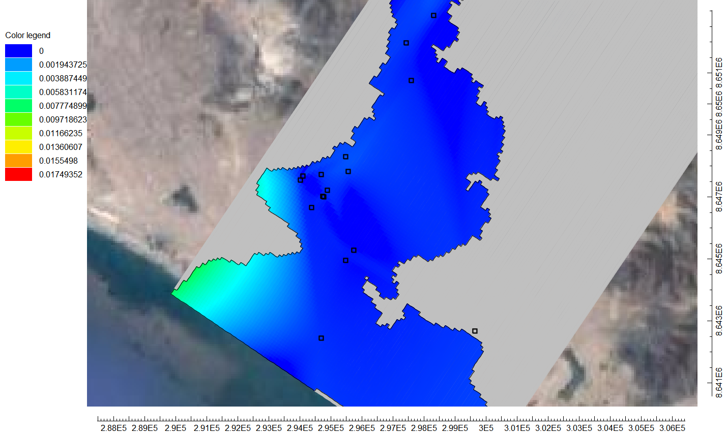
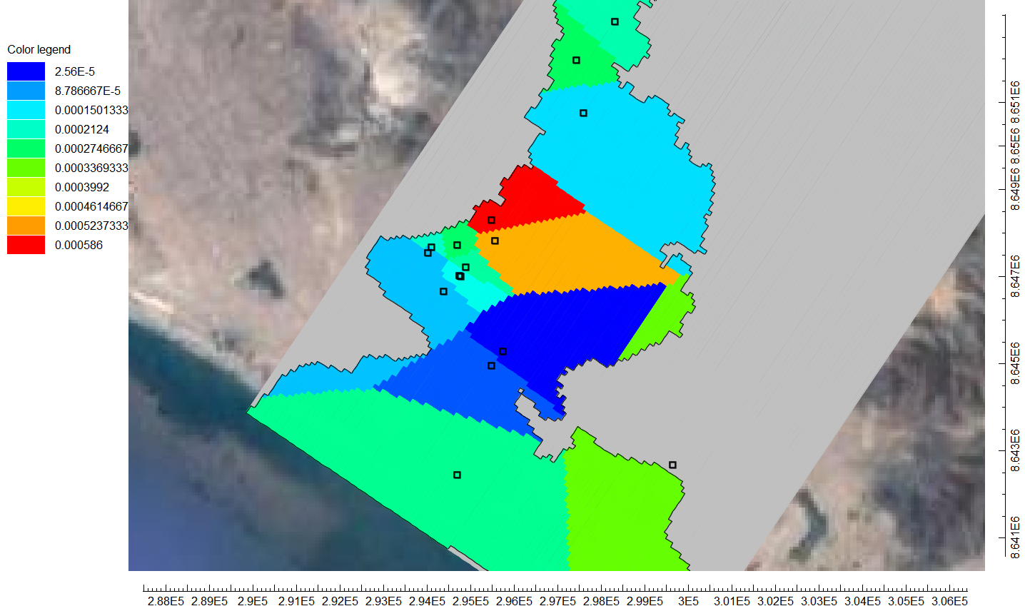
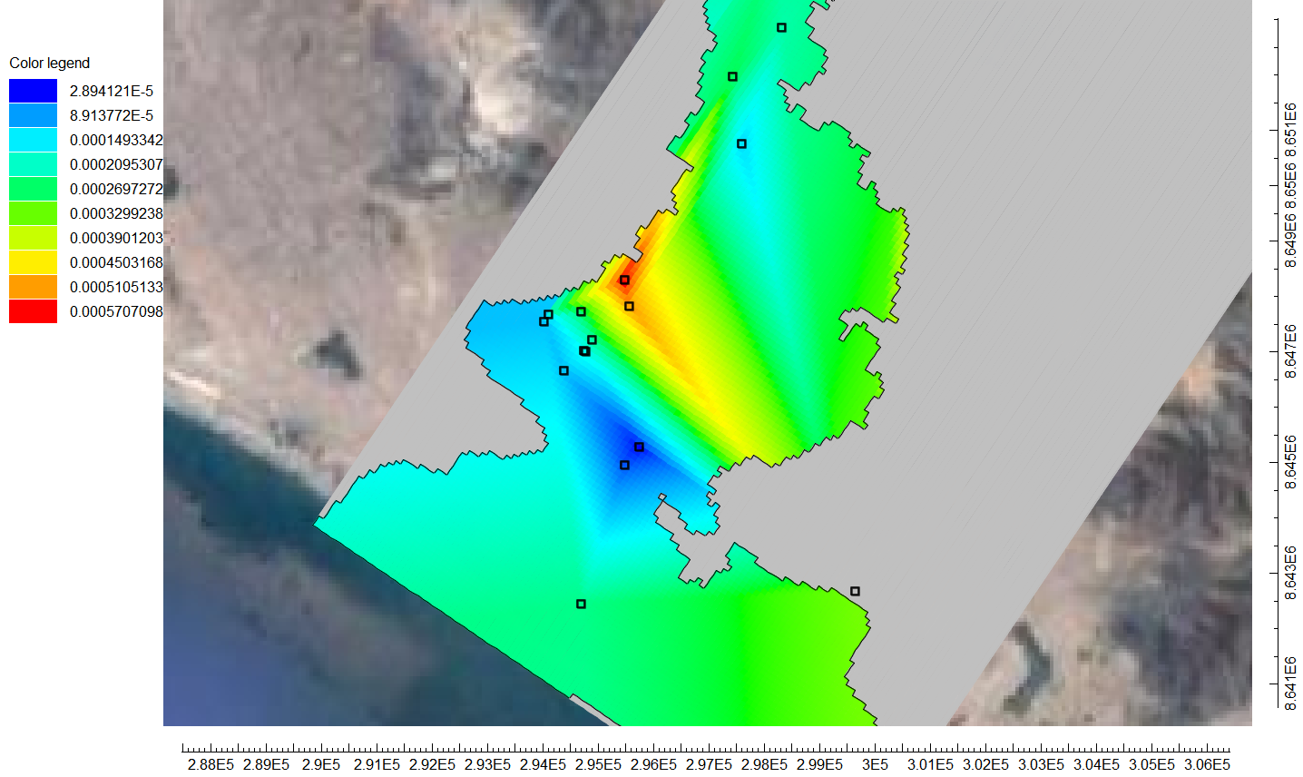
Some figures of the interpolated values from different methods for the hydraulic conductivity values on the active part of the model are shown below: