Introduction to Python and Geopandas for Flooded Area Analysis - Tutorial
/
Geopandas is one of the most advanced geospatial libraries in Python because it combines the spatial tools of Shapely, it can create and read different OGC vector spatial data, it can couple the Pandas tools to manage, filter, and make operations over the columns of the metadata, it has the capability to plot geospatial data on Matplotlib and even to Folium among other features. We have developed a tutorial of Geopandas applied to the analysis of flooded areas over the Boise city for a return period of 200 years; the tutorial covers introductory concepts of Geopandas, it will work with point, line and polygon vector data, create plots, simplify vertices and perform geospatial queries over inundated facilities and highways.
Tutorial
Code
import geopandas as gpd
import matplotlib.pyplot as plt
#open flooded areas
floodedAreas = gpd.read_file('../Data/Shps/boiseFlood200yr_v4.shp')
floodedAreas.head()| fid | STAGE | ELEV | USGSID | GRIDID | QCFS | STGRATING | Comments | Area | geometry | |
|---|---|---|---|---|---|---|---|---|---|---|
| 0 | 1.0 | 14.94 | 2617.892 | 13206000 | 13 | 23900 | EXTRAPOLATED, from USACE MODEL | 0.5-percent chance flow | 29243133 | POLYGON ((-116.30349 43.68274, -116.30350 43.6... |
#show columns
floodedAreas.columns
Index(['fid', 'STAGE', 'ELEV', 'USGSID', 'GRIDID', 'QCFS', 'STGRATING',
'Comments', 'Area', 'geometry'],
dtype='object')#show bounds per element
floodedAreas.bounds.head()| minx | miny | maxx | maxy | |
|---|---|---|---|---|
| 0 | -116.516417 | 43.662396 | -116.298905 | 43.694833 |
#plot geometry
floodedAreas.plot()
<AxesSubplot:>
#calculate areas
floodedAreasUtm = floodedAreas.to_crs(32611)
floodedAreasUtm['area'] = floodedAreasUtm.area
floodedAreasUtm['area_km2'] = floodedAreasUtm.area/1000000
floodedAreasUtm.head()| fid | STAGE | ELEV | USGSID | GRIDID | QCFS | STGRATING | Comments | Area | geometry | area | area_km2 | |
|---|---|---|---|---|---|---|---|---|---|---|---|---|
| 0 | 1.0 | 14.94 | 2617.892 | 13206000 | 13 | 23900 | EXTRAPOLATED, from USACE MODEL | 0.5-percent chance flow | 29243133 | POLYGON ((556138.632 4836872.248, 556138.373 4... | 2.922113e+07 | 29.221126 |
Working with linestrings
primaryHighways = gpd.read_file('../Data/Shps/primaryHighways.gpkg')
primaryHighways.head()| full_id | osm_id | osm_type | highway | old_name | maxspeed:variable | maxspeed:conditional | turn:lanes:both_ways | turn:lanes | turn:lanes:backward | ... | alt_name | old_ref | ref | oneway | maxspeed | NHS | lanes | surface | name | geometry | |
|---|---|---|---|---|---|---|---|---|---|---|---|---|---|---|---|---|---|---|---|---|---|
| 0 | w13691899 | 13691899 | way | primary | None | None | None | None | None | None | ... | None | None | None | None | None | None | None | asphalt | North Linder Road | LINESTRING (-116.41365 43.67338, -116.41365 43... |
| 1 | w13692173 | 13692173 | way | primary | None | None | None | None | None | None | ... | None | None | None | None | None | None | 4 | None | North Ten Mile Road | LINESTRING (-116.43362 43.66294, -116.43362 43... |
| 2 | w13692295 | 13692295 | way | primary | None | None | None | None | None | None | ... | None | None | ID 55 | yes | 55 mph | yes | None | asphalt | North Eagle Road | LINESTRING (-116.35424 43.64725, -116.35423 43... |
| 3 | w13695920 | 13695920 | way | primary | None | None | None | None | None | None | ... | None | US 30 | None | yes | 40 mph | None | None | paved | East Fairview Avenue | LINESTRING (-116.35642 43.61960, -116.35903 43... |
| 4 | w13696901 | 13696901 | way | primary | None | None | None | None | None | None | ... | North Horseshoe Bend Road | None | ID 55 | None | 55 mph | yes | None | asphalt | North Highway 55 | LINESTRING (-116.26604 43.76983, -116.26620 43... |
5 rows × 35 columns
#show column names
primaryHighways.columns
Index(['full_id', 'osm_id', 'osm_type', 'highway', 'old_name',
'maxspeed:variable', 'maxspeed:conditional', 'turn:lanes:both_ways',
'turn:lanes', 'turn:lanes:backward', 'turn:lanes:forward',
'official_name', 'maxspeed:type', 'cycleway', 'lanes:forward',
'lanes:both_ways', 'lanes:backward', 'layer', 'bridge',
'source:maxspeed', 'source:hgv:national_network',
'hgv:national_network', 'hgv', 'cycleway:right', 'bicycle', 'alt_name',
'old_ref', 'ref', 'oneway', 'maxspeed', 'NHS', 'lanes', 'surface',
'name', 'geometry'],
dtype='object')#show roads
primaryHighways['name'].value_counts()West Chinden Boulevard 38
West Fairview Avenue 34
West State Street 24
North Eagle Road 17
East Chinden Boulevard 16
East Fairview Avenue 12
South Eagle Road 12
North Highway 55 10
South Linder Road 10
East State Street 9
North Ten Mile Road 9
North Linder Road 8
North Glenwood Street 8
North Milwaukee Street 4
North Meridian Road 4
Emmett Highway 3
State Hwy 55 1
North Five Mile Road 1
West Cherry Lane 1
Name: name, dtype: int64# show figure with plotting options
fig, ax = plt.subplots(figsize=(16,16))
primaryHighways.plot(column='name', ax=ax, legend=True, categorical=True)<AxesSubplot:>
# show figure with plotting options with flooding area
fig, ax = plt.subplots(figsize=(16,16))
primaryHighways.plot(column='name', ax=ax, legend=True, categorical=True)
floodedAreas.plot(ax=ax, alpha=0.5)
<AxesSubplot:>
Working with polygons
primaryFacilities = gpd.read_file('../Data/Shps/schoolsHospitalsPoliceFire.gpkg')
primaryFacilities.head()| amenity | name | geometry | |
|---|---|---|---|
| 0 | school | Pioneer Elementary School | MULTIPOLYGON (((-116.34768 43.64752, -116.3475... |
| 1 | school | Centennial High School | MULTIPOLYGON (((-116.33940 43.65290, -116.3389... |
| 2 | school | Joplin Elementary School | MULTIPOLYGON (((-116.33274 43.65530, -116.3300... |
| 3 | school | Lowell Scott Middle School | MULTIPOLYGON (((-116.35409 43.65206, -116.3539... |
| 4 | school | Cecil D. Andrus Elementary School | MULTIPOLYGON (((-116.34585 43.66075, -116.3447... |
#show columns
primaryFacilities['amenity'].unique()
array(['school', 'hospital', 'fire_station'], dtype=object)#plot schools
fig, ax = plt.subplots(figsize=(16,16))
ax.axis('equal')
primaryFacilities.plot(column='amenity', ax=ax, legend=True, categorical=True, cmap='plasma')<AxesSubplot:>
#plot schools with flooded areas
fig, ax = plt.subplots(figsize=(16,16))
ax.axis('equal')
primaryFacilities.plot(column='amenity', ax=ax, legend=True, categorical=True, cmap='plasma')
floodedAreas.plot(ax=ax, alpha=0.5)
<AxesSubplot:>
Spatial operations
#show geoframe crs
print(floodedAreas.crs)
print(primaryHighways.crs)
print(primaryFacilities.crs)
epsg:4326
epsg:4326
epsg:4326#make composite plot
fig, ax = plt.subplots(figsize=(16,12))
flooded = floodedAreas.plot(ax=ax, alpha=0.5)
highways = primaryHighways.plot(column='name', ax=ax, categorical=True)
schools = primaryFacilities.plot(column='amenity', ax=ax, categorical=True, cmap='plasma')
ax.set_aspect('equal')
plt.show()
Plot data with Folium
All data need to be in geographical coordinates
# plot with folium
import folium

#convert everythin to WGS84
#floodedAreasGeo = floodedAreas.to_crs(4326)
#primaryHighwaysGeo = primaryHighwaysFix.to_crs(4326)
#schoolPointsGeo = schoolPoints.to_crs(4326)
#we need to have a reference centroid for the map
#dissolve flooded areas
floodedDissolved = floodedAreas.dissolve()
floodedDissolved| geometry | fid | STAGE | ELEV | USGSID | GRIDID | QCFS | STGRATING | Comments | Area | |
|---|---|---|---|---|---|---|---|---|---|---|
| 0 | POLYGON ((-116.30349 43.68274, -116.30350 43.6... | 1.0 | 14.94 | 2617.892 | 13206000 | 13 | 23900 | EXTRAPOLATED, from USACE MODEL | 0.5-percent chance flow | 29243133 |
#get reference coords to initialize the map
refX = floodedDissolved.centroid.x
refY = floodedDissolved.centroid.y

#create map
map = folium.Map(location = [refY,refX], tiles='OpenStreetMap', zoom_start = 13)
map
C:\Users\saulm\AppData\Local\Temp\ipykernel_2280\3149012135.py:2: UserWarning: Geometry is in a geographic CRS. Results from 'centroid' are likely incorrect. Use 'GeoSeries.to_crs()' to re-project geometries to a projected CRS before this operation.
refX = floodedDissolved.centroid.x
C:\Users\saulm\AppData\Local\Temp\ipykernel_2280\3149012135.py:3: UserWarning: Geometry is in a geographic CRS. Results from 'centroid' are likely incorrect. Use 'GeoSeries.to_crs()' to re-project geometries to a projected CRS before this operation.
refY = floodedDissolved.centroid.y#check the number of vertices of lines
import numpy as np
nVertexFlooded = [np.array(row.geometry.exterior.coords).shape[0] for index, row in floodedAreas.iterrows()]
nVertexHighways = [np.array(row.geometry.coords).shape[0] for index, row in primaryHighways.iterrows()]
print(sum(nVertexFlooded))
print(sum(nVertexHighways))41787
2280#a light version of the flooded areas
floodedAreasLight = floodedAreas.simplify(tolerance=0.0001)
nVertexFlooded = [np.array(row.exterior.coords).shape[0] for row in floodedAreasLight]
print(sum(nVertexFlooded))3250#create map
map = folium.Map(location = [refY,refX], tiles='OpenStreetMap', zoom_start = 12)
floodedJson = folium.GeoJson(data=floodedAreasLight.to_json(),
style_function=lambda x: {'fillColor': 'royalblue'})
primaryJson = folium.GeoJson(data=primaryHighways.to_json(),
style_function=lambda x: {'color': 'darkgreen'})
facilitiesJson = folium.GeoJson(data=primaryFacilities.to_json(),
style_function=lambda x: {'color': 'crimson'})
floodedJson.add_to(map)
primaryJson.add_to(map)
facilitiesJson.add_to(map)
mapClip and export flooded schools
#analyze schools that are flooded
for index, facility in primaryFacilities.iterrows():
    floodedStatus = floodedDissolved.intersects(facility.geometry)[0]
    print(floodedStatus)
    primaryFacilities.loc[index,'Flooded']=floodedStatus
False
False
False
False
False
False
False
False
False
True
False
False
False
False
False
False
False
False
False
False
True
False
False
False
False
FalsefloodedFacilities = primaryFacilities[primaryFacilities['Flooded']==True]
floodedFacilities.head()| amenity | name | geometry | Flooded | |
|---|---|---|---|---|
| 9 | hospital | Saint Alphonsus Eagle Health Plaza | MULTIPOLYGON (((-116.34898 43.68815, -116.3488... | True |
| 20 | hospital | None | MULTIPOLYGON (((-116.31779 43.68126, -116.3163... | True |
floodedFacilities.dtypesamenity object
name object
geometry geometry
Flooded object
dtype: object#export as geopackage
floodedFacilities['geometry'].to_file('../Out/floodedSchools.gpkg')Input data
You can download the input data from this link.