

Modeling Brine Density vs Concentration Regression Lines with Phreeqc and Aquifer App - Tutorial
/
Complex geochemical simulations are entirely possible to be performed with Phreeqc coupled with Aquifer App and Python. Brines can be simulated at different concentrations to obtain relations that are input of other variable density flow models. In this case we have model one brine, sodium bicarbonate, with the REACTION keyword with moles values that range from 0.5 to 12 moles. Values of mass, volume, concentration, and density were processed in Python from the dataframes generated from Aquifer App.
Tutorial
Code
Phreeqc input files:
TITLE Brine 1: Dissolved sodium bicarbonate
SOLUTION 2
        pH      7.0
        temp    25.0
REACTION 1
        NaHCO3		1.0
        0    0.5    1.0    2.0    4.0    6.0    8.0    10.0    12.0 moles
END
Python code
import pandas as pd
import numpy as np
import matplotlib.pyplot as plt
from scipy import stats
# open solution description dataframe
descDf = pd.read_csv('solutionDescription.csv')descDf.head()| Simulation | Type | Number | Parameter | Value | |
|---|---|---|---|---|---|
| 0 | 1 | initial | 1 | pH | 7.00000 |
| 1 | 1 | initial | 1 | pe | 4.00000 |
| 2 | 1 | initial | 1 | Specific Conductance (µS/cm, 25°C) | 0.00000 |
| 3 | 1 | initial | 1 | Density (g/cm³) | 0.99704 |
| 4 | 1 | initial | 1 | Volume (L) | 1.00297 |
# filter the density row and works only for the batch reactions and not for initial solution
densityDf = descDf[(descDf['Parameter']=='Density (g/cm³)')&(descDf['Type']=='batch')]
densityDf.head()| Simulation | Type | Number | Parameter | Value | |
|---|---|---|---|---|---|
| 18 | 1 | batch | 1 | Density (g/cm³) | 0.99704 |
| 33 | 1 | batch | 2 | Density (g/cm³) | 1.02698 |
| 49 | 1 | batch | 3 | Density (g/cm³) | 1.05628 |
| 65 | 1 | batch | 4 | Density (g/cm³) | 1.11283 |
| 81 | 1 | batch | 5 | Density (g/cm³) | 1.21767 |
# filter the volumne row and works only for the batch reactions and not for initial solution
volumeDf = descDf[(descDf['Parameter']=='Volume (L)')&(descDf['Type']=='batch')]
volumeDf.head()| Simulation | Type | Number | Parameter | Value | |
|---|---|---|---|---|---|
| 19 | 1 | batch | 1 | Volume (L) | 1.00297 |
| 34 | 1 | batch | 2 | Volume (L) | 1.01463 |
| 50 | 1 | batch | 3 | Volume (L) | 1.02625 |
| 66 | 1 | batch | 4 | Volume (L) | 1.04959 |
| 82 | 1 | batch | 5 | Volume (L) | 1.09721 |
# moles list
molAmount = [0.0, 0.5, 1.0, 2.0, 4.0, 6.0, 8.0, 10.0, 12.0]
#Working for the brine =
# brine data
index = 1
molarMass = 84.01 #g/mol
#filter the simulation for given index
brineDenDf = densityDf[densityDf['Simulation'] == index]
brineVolDf = volumeDf[volumeDf['Simulation'] == index]
#set batch reaction number as index
brineDenDf.index = brineDenDf['Number']
brineVolDf.index = brineVolDf['Number']
#order the batch in ascending order
brineDenDf = brineDenDf.sort_index(ascending=True)
brineVolDf = brineVolDf.sort_index(ascending=True)
#show the resulting dataframe
print(brineDenDf)
print(brineVolDf)Simulation Type Number Parameter Value
Number
1 1 batch 1 Density (g/cm³) 0.99704
2 1 batch 2 Density (g/cm³) 1.02698
3 1 batch 3 Density (g/cm³) 1.05628
4 1 batch 4 Density (g/cm³) 1.11283
5 1 batch 5 Density (g/cm³) 1.21767
6 1 batch 6 Density (g/cm³) 1.31205
7 1 batch 7 Density (g/cm³) 1.39662
8 1 batch 8 Density (g/cm³) 1.47210
9 1 batch 9 Density (g/cm³) 1.53917
Simulation Type Number Parameter Value
Number
1 1 batch 1 Volume (L) 1.00297
2 1 batch 2 Volume (L) 1.01463
3 1 batch 3 Volume (L) 1.02625
4 1 batch 4 Volume (L) 1.04959
5 1 batch 5 Volume (L) 1.09721
6 1 batch 6 Volume (L) 1.14634
7 1 batch 7 Volume (L) 1.19722
8 1 batch 8 Volume (L) 1.24998
9 1 batch 9 Volume (L) 1.30467#creation of another dataframe with for the concentration and densities
brineConDf = pd.DataFrame(index = brineDenDf.index)
brineConDf['mass(g)'] = np.asarray(molAmount) * molarMass
brineConDf['volume(L)'] = brineVolDf['Value']
brineConDf['concentration(g/L)'] = brineConDf['mass(g)'] / brineConDf['volume(L)']
brineConDf['density(g/cm³)'] = brineDenDf['Value']
print(brineConDf)mass(g) volume(L) concentration(g/L) density(g/cm³)
Number
1 0.000 1.00297 0.000000 0.99704
2 42.005 1.01463 41.399328 1.02698
3 84.010 1.02625 81.861145 1.05628
4 168.020 1.04959 160.081556 1.11283
5 336.040 1.09721 306.267715 1.21767
6 504.060 1.14634 439.712476 1.31205
7 672.080 1.19722 561.367167 1.39662
8 840.100 1.24998 672.090753 1.47210
9 1008.120 1.30467 772.701143 1.53917# Perform linear regression
slope, intercept, r_value, p_value, std_err = stats.linregress(brineConDf['concentration(g/L)'], brineConDf['density(g/cm³)'])
# Create the regression line
regression_line = slope * brineConDf['concentration(g/L)'] + intercept
#Create figure
fig = plt.figure(figsize=(12,6))
# Plot data points
plt.scatter(brineConDf['concentration(g/L)'], brineConDf['density(g/cm³)'], color='royalblue', label='Data points')
# Plot regression line
plt.plot(brineConDf['concentration(g/L)'], regression_line, color='teal', label='Regression line')
# Add regression formula and R-squared value to the plot
formula = f'y = {slope:.6f}x + {intercept:.2f}\n$R^2 = {r_value**2:.2f}$'
plt.text(300, 1, formula, fontsize=12, color='teal')
# Customize the plot
plt.xlabel('Concentration ((g/L)')
plt.ylabel('Density (g/cm³)')
plt.title('NaHCO3 Concentration vs Density')
plt.legend()
plt.grid(True)
# Show the plot
plt.show()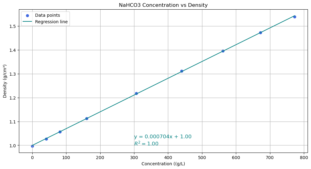
Input files
You can download the input data from this link.


