Plotting Water Surface Elevation from a 2D HEC-RAS Model using Python - Tutorial

This tutorial demonstrates how to accurately and efficiently extract the water surface elevation at a specific point from a HEC-RAS 2D unsteady flow model using Python in Jupyter Lab. Since water levels vary across the mesh and native software tools can limit automation, the author teaches how to open HDF5 output files (.hdf), load a point shapefile using GeoPandas, and apply a geospatial index K-d tree to locate the nearest computational cell. Finally, the time series data is processed to generate a water level hydrograph, which is essential for hydrogeological model calibration.

Tutorial

Code

#!pip install h5py geopandas

import h5py
import numpy as np
import pandas as pd
import geopandas as gpd
from scipy.spatial import KDTree
import matplotlib.pyplot as plt

hdfPath = '../HecUnsteady/theisNashUnsteady.p01.hdf'
AreaName = '2D Flow Area'

sw1Df = gpd.read_file('../Shp/SW1.shp')
sw1Coords = list(sw1Df.iloc[0].geometry.coords)[0]
sw1Coords

(697308.6910000006, 4345781.995000001)

hdf = h5py.File(hdfPath,'r')
cellCentroidsArray = np.asarray(hdf['Geometry']['2D Flow Areas']['Cell Points'])
cellCentroidsArray[:5]

array([[ 697293.70114532, 4345868.42012913],
       [ 697295.70114532, 4345868.42012913],
       [ 697289.70114532, 4345866.42012913],
       [ 697291.70114532, 4345866.42012913],
       [ 697293.70114532, 4345866.42012913]])

spatialIndex = KDTree(cellCentroidsArray)

timeBlocks = hdf['Results']['Unsteady']['Output']['Output Blocks']['Base Output']['Unsteady Time Series']['Time Date Stamp']
timeBlocksList = []
for timeBlock in timeBlocks:
    timeString = timeBlock.decode('utf-8').strip()
    timeDf = pd.to_datetime(timeString, format='%d%b%Y %H:%M:%S')
    timeBlocksList.append(timeDf)
timeBlocksList[:5]

[Timestamp('2023-01-15 00:00:00'),
 Timestamp('2023-01-15 04:00:00'),
 Timestamp('2023-01-15 08:00:00'),
 Timestamp('2023-01-15 12:00:00'),
 Timestamp('2023-01-15 16:00:00')]

surfaceDataset = hdf['Results']['Unsteady']['Output']['Output Blocks']['Base Output']['Unsteady Time Series']['2D Flow Areas']['Perimeter 1']['Water Surface']
surfaceDatasetArray = np.asarray(surfaceDataset)
surfaceDatasetArray[:2]

array([[149.05461, 149.05457, 149.05469, ..., 148.81921, 149.04991,
        148.80786],
       [149.561  , 149.56096, 149.56113, ..., 149.44379, 149.55418,
        149.4338 ]], shape=(2, 7908), dtype=float32)

surfaceDatasetArray.shape

(187, 7908)

distance, cellIndex = spatialIndex.query(sw1Coords)

print(distance)

1.077286895311947

print(cellIndex)

3978

#check position 
print(sw1Coords)
print(cellCentroidsArray[cellIndex])

(697308.6910000006, 4345781.995000001)
[ 697307.70114532 4345782.42012913]

#create modeled SW1 dataframe
sw1SimDf = pd.DataFrame()
sw1SimDf['Date'] = timeBlocksList
sw1SimDf['WSE'] = surfaceDatasetArray[:,cellIndex]
sw1SimDf = sw1SimDf.set_index(['Date'])
sw1SimDf.head()

	WSE
Date
2023-01-15 00:00:00	149.053177
2023-01-15 04:00:00	149.558655
2023-01-15 08:00:00	149.503647
2023-01-15 12:00:00	149.476654
2023-01-15 16:00:00	149.445267

fig, ax = plt.subplots()
sw1SimDf.plot(ax=ax)
ax.legend()
ax.grid()
ax.set_xlim(sw1SimDf.index[0], sw1SimDf.index[-1])

(464928.0, 465672.0)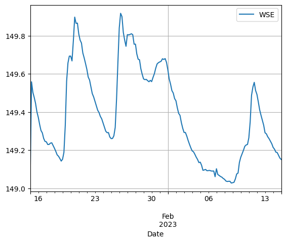

Input data

You can download the input data from this link:

owncloud.hatarilabs.com/s/LHpEe67q0kbYFCq

Password: Hatarilabs