Produced Water Chemistry and Isotope Analysis with Python and Pandas - Tutorial

On hydrocarbon extraction, water is a byproduct that comes from the geologic formations that have also oil and gas. Produced water can be defined as fossil water, or water with a high residence time on the earth, with a particular water chemistry that is important to analyze when we deal with the treatment methods, disposal techniques or safety to drinking water sources. The USGS has developed a produced water geochemical database with more than 100K points that includes spatial information, well description, rock properties, water chemistry and isotopes.

Know more about the U.S. Geological Survey National Produced Waters Geochemical Database v2.3 on this link:

https://www.sciencebase.gov/catalog/item/59d25d63e4b05fe04cc235f9

Tutorial

Scripts

The scripting part for this tutorial is divided on two parts: Water Chemistry and Isotope Analysis:

---

Water Chemistry

#import required libraries
%matplotlib inline
import pandas as pd
import numpy as np
import matplotlib.pyplot as plt
import mplleaflet

#Open the USGS Produced Water Geochemical Database as a Pandas Dataframe
prodWatDf = pd.read_csv('../Csv/USGSPWDBv2.3n.csv', low_memory=False)
#Get the column headers
print(prodWatDf.keys())
#Get number of samples
print(prodWatDf.count()[:10])

Index(['IDUSGS', 'IDORIG', 'IDDB', 'SOURCE', 'REFERENCE', 'LATITUDE',
       'LONGITUDE', 'LATLONGAPX', 'API', 'USGSREGION',
       ...
       'Sr87Sr86', 'I129', 'Rn222', 'Ra226', 'Ra228', 'cull_PH', 'cull_MgCa',
       'cull_KCl', 'cull_K5Na', 'cull_chargeb'],
      dtype='object', length=190)
IDUSGS        114943
IDORIG        114943
IDDB          114943
SOURCE         75708
REFERENCE       7008
LATITUDE      103916
LONGITUDE     104179
LATLONGAPX     22611
API            74052
USGSREGION    114943
dtype: int64

#Total spatial distribution of samples
plt.scatter(prodWatDf.LONGITUDE,prodWatDf.LATITUDE)

<matplotlib.collections.PathCollection at 0x1a400054160>

---

Analysis of well depth (ft) distribution

#Description of the well depth database
prodWatDf.DEPTHWELL.describe()

count    42979.000000
mean      6760.011429
std       3336.825591
min         14.400000
25%       4158.000000
50%       6415.000000
75%       8915.000000
max      23258.000000
Name: DEPTHWELL, dtype: float64

#Histogram of well depth
prodWatDf.DEPTHWELL.hist()

<matplotlib.axes._subplots.AxesSubplot at 0x1a4002a3208>

---

Analysis of main components

# Boxplot of key components
fig = plt.plot(figsize=(12,8))
prodWatDf[prodWatDf.Ba<100][['As','Ba','Cd','Hg','Pb']].boxplot()
plt.ylim(0,80)
plt.show()

# Boxplot of key components with semilog y axis
fig = plt.plot(figsize=(12,8))
prodWatDf[prodWatDf.Ba<100][['As','Ba','Cd','Hg','Pb']].boxplot()
plt.ylim(0.00001,1000)
plt.semilogy()
plt.show()

---

Analysis of Arsenic distribution

prodWatDf.As.describe()

count    493.000000
mean       0.496993
std        1.035728
min        0.000070
25%        0.010000
50%        0.066000
75%        0.340000
max        7.000000
Name: As, dtype: float64

#Histogram of Arsenic concentrations
prodWatDf.As.hist(bins=20)

<matplotlib.axes._subplots.AxesSubplot at 0x1a400683c18>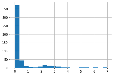

#Depth histogram of well with concentrations of Arsenic more than 0.1 mg/l
prodWatDf.DEPTHUPPER[prodWatDf.As > 0.1].hist()

<matplotlib.axes._subplots.AxesSubplot at 0x1a4003e2d68>

#Get the Geological Era and Period of samples with high Arsenic concentrations
asDf = prodWatDf[prodWatDf.As>0.1]
print(asDf.ERA.unique())
print(asDf.PERIOD.unique())

['Unknown' 'Paleozoic']
['Unknown' 'Devonian, M' 'Mississippian' 'Devonian, U - Mississippian, L']

#Spatial distribution of samples with high Arsenic concentrations
plt.scatter(asDf.LONGITUDE,asDf.LATITUDE,s=asDf.As*10)
mplleaflet.display()

C:\Users\Gida\Anaconda3\lib\site-packages\IPython\core\display.py:694: UserWarning: Consider using IPython.display.IFrame instead
  warnings.warn("Consider using IPython.display.IFrame instead")

---

Analysis of Barium distribution

#Statistical distribution of Barium values
prodWatDf.Ba.describe()

count    12498.000000
mean       134.621723
std        705.856150
min          0.000856
25%          3.000000
50%         14.708432
75%         65.690000
max      22400.000000
Name: Ba, dtype: float64

#Get the Geological Era and Period of samples with high Barium concentrations
baDf = prodWatDf[prodWatDf.Ba>14]
print(baDf.ERA.unique())
print(baDf.PERIOD.unique())

['Paleozoic' 'Mesozoic' 'Cenozoic' 'Unknown']
['Devonian, M' 'Permian (Leonardian)' 'Pennsylvanian' 'Cretaceous'
 'Paleogene' 'Neogene' 'Jurassic' 'Unknown' 'Devonian, U' 'Devonian'
 'Devonian, L' 'Silurian, L' 'Mississippian, L - Pennsylvanian, L'
 'Mississippian, L' 'Mississippian, U' 'Pennsylvanian, L'
 'Pennsylvanian, M' 'Silurian, U' 'Mississippian' 'Cambrian - Ordovician'
 'Silurian, U - Devonian, L' 'Jurassic - Cretaceous' 'Silurian'
 'Mississippian - Pennsylvanian' 'Ordovician, U - Silurian, L' 'Tertiary'
 'Permian' 'Cambrian' 'Ordovician' 'Triassic']

#Spatial distribution of samples with high Barium concentrations
plt.scatter(baDf.LONGITUDE,baDf.LATITUDE,s=baDf.Ba/100)
plt.ylim(25,50)
plt.xlim(-130,-75)

(-130, -75)

---

Analysis of Cadmium distribution

#Get the Geological Era and Period of samples with high Cadmium concentrations
cdDf = prodWatDf[prodWatDf.Cd>0.01]
print(cdDf.ERA.unique())
print(cdDf.PERIOD.unique())

['Unknown' 'Paleozoic']
['Unknown' 'Devonian, M' 'Devonian, U - Mississippian, L']

prodWatDf.Cd[prodWatDf.Cd<2].hist()

<matplotlib.axes._subplots.AxesSubplot at 0x1a4003d1470>

#Spatial distribution of samples with high Cadmium concentrations
plt.scatter(cdDf.LONGITUDE,cdDf.LATITUDE,s=cdDf.Cd*10)
plt.ylim(25,50)
plt.xlim(-130,-75)
mplleaflet.display()

#We can notice that Arsenic and Cadmium are spatially correlated, lets analyze their concentration correlation
plt.scatter(prodWatDf.As,prodWatDf.Cd)
plt.xlim(0,1)
plt.ylim(0,0.3)
plt.xlabel('Arsenic')
plt.ylabel('Cadmium')

Text(0, 0.5, 'Cadmium')

#Correlation is not that great, but there is a group of high concentration of Arsenic

---

Analysis of Mercury distribution

#Get the Geological Era and Period of samples with high Mercury concentrations
hgDf = prodWatDf[prodWatDf.Hg>0.0001]
print(hgDf.ERA.unique())
print(hgDf.PERIOD.unique())

['Unknown' 'Paleozoic']
['Unknown' 'Devonian, M']

hgDf.PERIOD.describe()

count         145
unique          2
top       Unknown
freq           80
Name: PERIOD, dtype: object

---

Analysis of Lead distribution

prodWatDf.Pb.describe()

count     359.000000
mean       29.586492
std       432.145200
min         0.000120
25%         0.007900
50%         0.030000
75%         0.215000
max      8187.000000
Name: Pb, dtype: float64

#Get the Geological Era and Period of samples with high Lead concentrations
pbDf = prodWatDf[prodWatDf.Pb>1]
print(pbDf.ERA.unique())
print(pbDf.PERIOD.unique())

['Paleozoic' 'Unknown' 'Mesozoic']
['Devonian, U - Mississippian, L' 'Unknown' 'Jurassic' 'Cretaceous'
 'Devonian']

pbDf.Pb[pbDf.Pb<100].hist()

<matplotlib.axes._subplots.AxesSubplot at 0x1a400ba37b8>

#Spatial distribution of samples with high Lead concentrations
import numpy as np
plt.scatter(pbDf.LONGITUDE,pbDf.LATITUDE,s=np.log10(pbDf.Pb)*40)

<matplotlib.collections.PathCollection at 0x1a400cb8828>

---

Isotope Analysis

#import required libraries
%matplotlib inline
import matplotlib.pyplot as plt
import pandas as pd
import numpy as np

#Open the USGS Produced Water Geochemical Database as a Pandas Dataframe
prodWatDf = pd.read_csv('../Csv/USGSPWDBv2.3n.csv', low_memory=False)
prodWatDf.loc[:,['IDORIG','dD','d18O']].describe()

	dD	d18O
count	1039.000000	1335.000000
mean	-37.198499	-0.725832
std	33.966057	6.684780
min	-148.300000	-18.000000
25%	-49.050000	-4.600000
50%	-35.000000	-0.520000
75%	-16.990000	4.300000
max	61.220000	18.000000

#create array and equation application
delta18O = np.linspace(-20,20,num=50)
delta2H = delta18O*8.13+10.8
delta2H[:5]

array([-151.8       , -145.16326531, -138.52653061, -131.88979592,
       -125.25306122])

prodWatDf.ERA.unique()

array(['Paleozoic', 'Unknown', 'Mesozoic', 'Cenozoic', 'Proterozoic'],
      dtype=object)

#Isotope representation
fig, ax1 = plt.subplots(figsize=(12,8))

proteoDf = prodWatDf[prodWatDf.ERA=='Proterozoic']
ax1.scatter(proteoDf.d18O,proteoDf.dD,marker='o',alpha=0.9,label='Proterozoic')

paleoDf = prodWatDf[prodWatDf.ERA=='Paleozoic']
ax1.scatter(paleoDf.d18O,paleoDf.dD,marker='o',alpha=0.7,label='Paleozoic')

mesoDf = prodWatDf[prodWatDf.ERA=='Mesozoic']
ax1.scatter(mesoDf.d18O,mesoDf.dD,marker='o',alpha=0.5,label='Mesozoic')

cenoDf = prodWatDf[prodWatDf.ERA=='Cenozoic']
ax1.scatter(cenoDf.d18O,cenoDf.dD,marker='o',alpha=0.3,label='Cenozoic')

ax1.plot(delta18O,delta2H,label='GMWL')
ax1.set_xlabel('δ18O 0/00 VSMOW')
ax1.set_ylabel('δ2H 0/00 VSMOW')
plt.legend()

<matplotlib.legend.Legend at 0x1fe010d1940>

---

Input files

You can download the input files for this tutorial here.