This is an applied example of a fully geospatial groundwater flow model with the MODFLOW 6 Disv discretized by vertices option. Model was constructed with Python and Flopy from a series of shapefiles and it has a progressive refinement for well and river boundary conditions. Regional flow has been simulated as a General Head Boundary and plotting options were developed for the grid and model output representation on areal view and cross section.

Tutorial

Code

Import the required packages

#import basic packages
import os, json
import pandas as pd
import numpy as np

#import geospatial packages
import rasterio
import geopandas as gpd
from shapely.geometry import Polygon, Point, MultiLineString, MultiPoint

#plots
import matplotlib.pyplot as plt

#modflow
import flopy
import flopy.discretization as fgrid
import flopy.plot as fplot
from flopy.utils.gridintersect import GridIntersect
import flopy.utils.binaryfile as bf

#link path to src folder
import sys
sys.path.insert(0, '../src')
from meshProperties import mesh_shape
from geoVoronoi import createVoronoi

Define mesh

Build mesh from geospatial data with a given src.

#Create mesh object
vorMesh = createVoronoi()

#Define base refinement and refinement levels
vorMesh.defineParameters(maxRef = 80, minRef=10, stages=5)

/--------Sumary of cell discretization-------/
Maximun refinement: 80.00 m.
Minimum refinement: 10.00 m.
Cell size list: [80.  62.5 45.  27.5 10. ] m.
/--------------------------------------------/

#Open limit layers and refinement definition layers
vorMesh.addLimit('basin','../in/shp/ModelLimit1.shp')
vorMesh.addLayer('wells','../in/shp/ModelWell2.shp')
vorMesh.addLayer('river','../in/shp/ModelRiver2.shp')

#Generate point pair array
vorMesh.extractOrgVertices()

#Generate the point cloud and voronoi
vorMesh.createPointCloud()
vorMesh.generateVoronoi()

#check or create an output folder
outPath = '../out'
if os.path.isdir(outPath):
    print('The output folder %s exists'%outPath)
else:
    os.mkdir(outPath)
    print('The output folder %s has been generated.'%outPath)

#Export point data and voronoi polygons
#Points
vorMesh.getPointsAsShp('vertexOrg',outPath+'/vertexOrg.shp')
vorMesh.getPointsAsShp('vertexDist',outPath+'/vertexDist.shp')
vorMesh.getPointsAsShp('vertexBuffer',outPath+'/vertexBuffer.shp')
vorMesh.getPointsAsShp('vertexMaxRef',outPath+'/vertexMaxRef.shp')
vorMesh.getPointsAsShp('vertexMinRef',outPath+'/vertexMinRef.shp')
vorMesh.getPointsAsShp('vertexTotal',outPath+'/vertexTotal.shp')
#Polygons

vorMesh.getPolyAsShp('voronoiRegions',outPath+'/voronoiRegions.shp')

/----Sumary of points for voronoi meshing----/
Distributed points from layers: 680
Points from layer buffers: 1360
Points from max refinement areas: 749
Points from min refinement areas: 1335
Total points inside the limit: 4090
/--------------------------------------------/

Time required for point generation: 2.12 seconds 

The output folder ../out exists

# plot geospatial data with geopandas
import warnings
warnings.filterwarnings('ignore')

voronoiMesh = gpd.read_file('../out/voronoiRegions.shp')
modelRiver = gpd.read_file('../in/shp/ModelRiver2.shp')
modelGhb = gpd.read_file('../in/shp/ModelGHB1.shp')
modelWell = gpd.read_file('../in/shp/ModelWell2.shp')

fig, ax = plt.subplots(figsize=(24,18))
voronoiMesh.plot(ax=ax, alpha=0.2, ec='grey', fc='crimson')
modelRiver.plot(ax=ax, alpha=0.6, ec='slateblue')
modelGhb.plot(ax=ax, alpha=0.6, ec='darkslategrey', lw=5)
modelWell.plot(ax=ax, alpha=0.6, fc='indigo',markersize=100)
plt.show()

Generation of the Voronoi grid

# get the mesh data from the shapefile
mesh=mesh_shape('../out/voronoiRegions.shp')
gridprops=mesh.get_gridprops_disv()

Creating a unique list of vertices [[x1,y1],[x2,y2],...]


100%|███████████████████████████████████████████████████████████████████████████| 4090/4090 [00:00<00:00, 31462.55it/s]


Extracting cell2d data and grid index



100%|████████████████████████████████████████████████████████████████████████████| 4090/4090 [00:01<00:00, 2332.42it/s]

#define the disv list of vertices and cells
cell2d = gridprops['cell2d']
vertices = gridprops['vertices']
ncpl = gridprops['ncpl']
nvert = gridprops['nvert']
centroids=gridprops['centroids']

#sample of the cell2d items
cell2d[:5]

[[0, 353305.0842893986, 8548677.699736858, 6, 35, 17, 18, 41, 38, 35],
 [1, 353314.9830338129, 8548668.095507141, 7, 35, 38, 54, 56, 50, 37, 35],
 [2, 353304.6801875851, 8548592.884968264, 5, 42, 34, 10, 11, 42],
 [3, 353325.0, 8547990.0, 5, 109, 108, 1, 2, 109],
 [4, 353305.0450244283, 8548666.712527014, 6, 35, 37, 36, 16, 17, 35]]

Define aquifer geometry

#Extract dem values for each centroid of the voronois
src = rasterio.open('../in/rst/ModeloDem1Filled.tif')
elevation=[x for x in src.sample(centroids)]

#number of lays
nlay = 3

#define mtop
mtop=np.array([elev[0] for i,elev in enumerate(elevation)])

#define zbot
zbot=np.zeros((nlay,ncpl))

AcuifInf_Bottom = -120
AcuifMed_Bottom = AcuifInf_Bottom + (0.5 * (mtop - AcuifInf_Bottom))
AcuifSup_Bottom = AcuifInf_Bottom + (0.75 * (mtop - AcuifInf_Bottom))

zbot[0,] = AcuifSup_Bottom 
zbot[1,] = AcuifMed_Bottom
zbot[2,] = AcuifInf_Bottom

Define a MODFLOW 6 simulation and model

# create simulation
model_name = 'geo_model'
model_ws = '../out/model'
exe_name = '../exe/mf6.exe'

sim = flopy.mf6.MFSimulation(sim_name=model_name, version='mf6', exe_name=exe_name,sim_ws=model_ws)

# create temporal discretization package - tdis
nper = 11
tdis_rc = [(1.0,1,1.0)] + [(200 * 86400.0, 4, 1.0) for a in range(nper -1)]

tdis=flopy.mf6.ModflowTdis(sim, nper=nper, time_units='seconds',perioddata=tdis_rc)

# create iterative model solution and register the gwf model with it
ims = flopy.mf6.ModflowIms(sim, linear_acceleration='BICGSTAB')

# create gwf model
gwf = flopy.mf6.ModflowGwf(sim, modelname=model_name, save_flows=True, newtonoptions=['under_relaxation'])

# disv
disv = flopy.mf6.ModflowGwfdisv(gwf, nlay=nlay, ncpl=ncpl,top=mtop, botm=zbot,nvert=nvert, vertices=vertices,cell2d=cell2d)

WARNING: Unable to resolve dimension of ('gwf6', 'disv', 'cell2d', 'cell2d', 'icvert') based on shape "ncvert".

ic = flopy.mf6.ModflowGwfic(gwf, strt=np.stack([mtop for i in range(nlay)]))

Define steady and transient parameters

Kx =[1E-5,5E-4,2E-4]
icelltype = [1,1,0]
npf = flopy.mf6.ModflowGwfnpf(gwf,save_specific_discharge=True,icelltype=icelltype,k=Kx)

sto=flopy.mf6.ModflowGwfsto(gwf,ss=1e-05, sy=0.15)

Plot grid from flopy utilities

#map view
fig = plt.figure(figsize=(18,12))
ax = fig.add_subplot(1, 1, 1, aspect='equal')
modelmap = flopy.plot.PlotMapView(model=gwf)
linecollection = modelmap.plot_grid(linewidth=0.5, color='royalblue')

#plot cross section
line = np.array([(353304.219,8548577.580), (356374.790,8548586.576)])

fig = plt.figure(figsize=(18, 6))
ax = fig.add_subplot(1, 1, 1, aspect='equal')
modelxsect = flopy.plot.PlotCrossSection(model=gwf, line={"line": line})
linecollection = modelxsect.plot_grid()

Evapotranspiration package

#evapotranspiration package
evtr = 1.2/365/86400
evt = flopy.mf6.ModflowGwfevta(gwf,ievt=1,surface=mtop,rate=evtr,depth=1.0)

Recharge package

#define a grid intersect object
tgr = fgrid.VertexGrid(vertices, cell2d)
ix2 = GridIntersect(tgr)

#find cells inside a polygon shapefile
zone1=gpd.read_file('../in/shp/ModelRechargeZone1.shp')
result=ix2.intersect(zone1['geometry'].loc[0])

#plot intersected cells
fig = plt.figure(figsize=(18,12))
ax = fig.add_subplot(1, 1, 1, aspect='equal')
pmv = fplot.PlotMapView(ax=ax, modelgrid=tgr)
pmv.plot_grid()
ix2.plot_polygon(result, ax=ax, fc='aqua', lw=3)

for cellid in result.cellids:
    (h2,) = ax.plot(
        tgr.xcellcenters[cellid],
        tgr.ycellcenters[cellid],
        "bo",
        alpha=0.5)

#apply recharge on selected cells
rchr = 0.2/365/86400
rchr_list = []
for i in result.cellids:
    rchr_list.append([0,i,rchr])
rchr_spd = {0:rchr_list}

#recharge package
rch = flopy.mf6.ModflowGwfrch(gwf, stress_period_data=rchr_spd)

Well package

#read well shapefile
well_zone=gpd.read_file('../in/shp/ModelWell2.shp')

#create list of well positions
list_wells=[]
for i in range(well_zone.shape[0]): 
    list_wells.append(well_zone['geometry'].loc[i])

#define multipoint geometry and intersect
mp = MultiPoint(points=list_wells)
result=ix2.intersect(mp)

#define pumping and apply to cells
pump = -0.15
well_list = []
for i in result.cellids:
    well_list.append([1,i,pump])
well_spd = {1:well_list}

#apply well package
well=flopy.mf6.ModflowGwfwel(gwf,stress_period_data=well_spd)

River package - RIV

#open river shapefile
river_zone=gpd.read_file('../in/shp/ModelRiver2.shp')

#intersect river geometry
result=ix2.intersect(river_zone['geometry'].loc[0])

#apply parameters to intersect cells
river_list = []
for i in result.cellids:
    river_list.append([0,i,mtop[i],0.01,mtop[i]-1])
river_spd = {0:river_list}

#create river package
river=flopy.mf6.ModflowGwfriv(gwf,stress_period_data=river_spd)

Regional flow as General Head Boundary - GHB

#open GHB file
boundaries_zone=gpd.read_file('../in/shp/ModelGHB1.shp')

#create list of geometries
list_boundaries=[]
for i in range(boundaries_zone.shape[0]):   
    list_boundaries.append(boundaries_zone['geometry'].loc[i])

#create multiline
mls = MultiLineString(lines=list_boundaries)

#intersect rivers with our grid
result=ix2.intersect(mls)

#define cell as ghb
#[cellid, bhead, cond, aux, boundname]
ghb_list=[]

for idx in result.cellids:
    point=centroids[idx]
    if point[0]<354500:
         ghb_list.append([0,i,55,0.01])
    else:
         ghb_list.append([0,i,90,0.01])
ghb_spd={0:ghb_list}

#define ghb package
ghb=flopy.mf6.ModflowGwfghb(gwf,stress_period_data=ghb_spd)

Define output and run simulation

hname = '{}.hds'.format(model_name)
cname = '{}.cbc'.format(model_name)
oc = flopy.mf6.ModflowGwfoc(gwf, budget_filerecord=cname,
 head_filerecord=hname,
 saverecord=[('HEAD', 'ALL'), ('BUDGET',
'ALL')])

sim.write_simulation()
sim.run_simulation()

writing simulation...
  writing simulation name file...
  writing simulation tdis package...
  writing ims package ims_-1...
  writing model geo_model...
    writing model name file...
    writing package disv...
    writing package ic...
    writing package npf...
    writing package sto...
    writing package evta_0...
    writing package rch_0...
INFORMATION: maxbound in ('gwf6', 'rch', 'dimensions') changed to 1142 based on size of stress_period_data
    writing package wel_0...
INFORMATION: maxbound in ('gwf6', 'wel', 'dimensions') changed to 3 based on size of stress_period_data
    writing package riv_0...
INFORMATION: maxbound in ('gwf6', 'riv', 'dimensions') changed to 2012 based on size of stress_period_data
    writing package ghb_0...
INFORMATION: maxbound in ('gwf6', 'ghb', 'dimensions') changed to 34 based on size of stress_period_data
    writing package oc...
FloPy is using the following executable to run the model: ../exe/mf6.exe
                                   MODFLOW 6
                U.S. GEOLOGICAL SURVEY MODULAR HYDROLOGIC MODEL
                            VERSION 6.3.0 03/04/2022

   MODFLOW 6 compiled Mar 02 2022 15:29:04 with Intel(R) Fortran Intel(R) 64
   Compiler Classic for applications running on Intel(R) 64, Version 2021.5.0
                             Build 20211109_000000

This software has been approved for release by the U.S. Geological 
Survey (USGS). Although the software has been subjected to rigorous 
review, the USGS reserves the right to update the software as needed 
pursuant to further analysis and review. No warranty, expressed or 
implied, is made by the USGS or the U.S. Government as to the 
functionality of the software and related material nor shall the 
fact of release constitute any such warranty. Furthermore, the 
software is released on condition that neither the USGS nor the U.S. 
Government shall be held liable for any damages resulting from its 
authorized or unauthorized use. Also refer to the USGS Water 
Resources Software User Rights Notice for complete use, copyright, 
and distribution information.


 Run start date and time (yyyy/mm/dd hh:mm:ss): 2022/06/06 14:44:30

 Writing simulation list file: mfsim.lst
 Using Simulation name file: mfsim.nam

    Solving:  Stress period:     1    Time step:     1
    Solving:  Stress period:     2    Time step:     1
    Solving:  Stress period:     2    Time step:     2
    Solving:  Stress period:     2    Time step:     3
    Solving:  Stress period:     2    Time step:     4
    Solving:  Stress period:     3    Time step:     1
    Solving:  Stress period:     3    Time step:     2
    Solving:  Stress period:     3    Time step:     3
    Solving:  Stress period:     3    Time step:     4
    Solving:  Stress period:     4    Time step:     1
    Solving:  Stress period:     4    Time step:     2
    Solving:  Stress period:     4    Time step:     3
    Solving:  Stress period:     4    Time step:     4
    Solving:  Stress period:     5    Time step:     1
    Solving:  Stress period:     5    Time step:     2
    Solving:  Stress period:     5    Time step:     3
    Solving:  Stress period:     5    Time step:     4
    Solving:  Stress period:     6    Time step:     1
    Solving:  Stress period:     6    Time step:     2
    Solving:  Stress period:     6    Time step:     3
    Solving:  Stress period:     6    Time step:     4
    Solving:  Stress period:     7    Time step:     1
    Solving:  Stress period:     7    Time step:     2
    Solving:  Stress period:     7    Time step:     3
    Solving:  Stress period:     7    Time step:     4
    Solving:  Stress period:     8    Time step:     1
    Solving:  Stress period:     8    Time step:     2
    Solving:  Stress period:     8    Time step:     3
    Solving:  Stress period:     8    Time step:     4
    Solving:  Stress period:     9    Time step:     1
    Solving:  Stress period:     9    Time step:     2
    Solving:  Stress period:     9    Time step:     3
    Solving:  Stress period:     9    Time step:     4
    Solving:  Stress period:    10    Time step:     1
    Solving:  Stress period:    10    Time step:     2
    Solving:  Stress period:    10    Time step:     3
    Solving:  Stress period:    10    Time step:     4
    Solving:  Stress period:    11    Time step:     1
    Solving:  Stress period:    11    Time step:     2
    Solving:  Stress period:    11    Time step:     3
    Solving:  Stress period:    11    Time step:     4

 Run end date and time (yyyy/mm/dd hh:mm:ss): 2022/06/06 14:44:36
 Elapsed run time:  5.962 Seconds

 Normal termination of simulation.





(True, [])

Plot model output

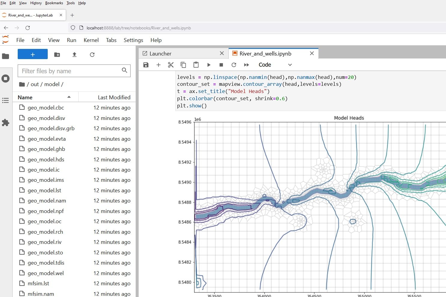
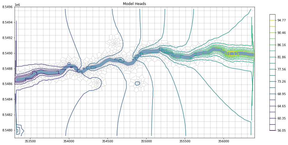
#open head file
hds = bf.HeadFile(model_ws+'/'+model_name + '.hds')
head = hds.get_data(totim=hds.get_times()[-1])
head[head==1e+30]=np.nan

#plot model heads
fig = plt.figure(figsize=(18, 12))
ax = fig.add_subplot(1, 1, 1, aspect='equal')
mapview = flopy.plot.PlotMapView(model=gwf)
modelRiver.plot(ax=ax, alpha=0.6, ec='slateblue')
linecollection = mapview.plot_grid(lw=0.2)

levels = np.linspace(np.nanmin(head),np.nanmax(head),num=20)
contour_set = mapview.contour_array(head,levels=levels)
t = ax.set_title("Model Heads")
plt.colorbar(contour_set, shrink=0.6)
plt.show()

#plot model heads with colorgrid and label contours
fig = plt.figure(figsize=(18, 12))
ax = fig.add_subplot(1, 1, 1, aspect='equal')
mapview = flopy.plot.PlotMapView(model=gwf)

quadmesh = mapview.plot_array(head, alpha=0.5)
levels = np.linspace(np.nanmin(head),np.nanmax(head),num=20)
c = mapview.contour_array(head, linewidths=0.75,colors='white',levels=levels)
plt.clabel(c, fmt='%3d')
plt.colorbar(quadmesh, shrink=0.6)
plt.show()

#plot cross section
fig = plt.figure(figsize=(18, 5))
ax = fig.add_subplot(1, 1, 1)
ax.set_title("plot_array()")

xsect = flopy.plot.PlotCrossSection(model=gwf, line={"line": line})
patch_collection = xsect.plot_array(head, head=head, alpha=0.5)
line_collection = xsect.plot_grid()
cb = plt.colorbar(patch_collection, shrink=0.75)

Input data

You can download the input data from this link.

Blog

River-Well-Aquifer Geospatial Groundwater Flow Model with Voronoi Mesh - Tutorial

Tutorial

Code

Import the required packages

Define mesh

Generation of the Voronoi grid

Define aquifer geometry

Define a MODFLOW 6 simulation and model

Define steady and transient parameters

Plot grid from flopy utilities

Evapotranspiration package

Recharge package

Well package

River package - RIV

Regional flow as General Head Boundary - GHB

Define output and run simulation

Plot model output

Input data

Hatari Labs

Our courses:

Blog

Tutorial

Code

Import the required packages

Define mesh

Generation of the Voronoi grid

Define aquifer geometry

Define a MODFLOW 6 simulation and model

Define steady and transient parameters

Plot grid from flopy utilities

Evapotranspiration package

Recharge package

Well package

River package - RIV

Regional flow as General Head Boundary - GHB

Define output and run simulation

Plot model output

Input data

Hatari Labs

Our courses:

Follow Us

Join us on social media for the latest webinars, tutorials and courses.