Smart analysis of online temperature sensor data with SensorThingsAPI and Python - Tutorial

This tutorial demonstrates how to connect to a SensorThings API FROST server using Python to retrieve, inspect, and visualize IoT sensor datastreams. After setting up the server connection and querying datastream details such as units and observation counts, the notebook extracts time-series observations using paginated REST requests and loads them into a Pandas DataFrame. Following the data preparation phase, the script produces a series of continuous time-series line charts using Matplotlib and Seaborn, displaying the chronological trend of air temperature measurements recorded over time.

Tutorial

Code

# Define conexion with the server

import requests
import pandas as pd
import matplotlib.pyplot as plt
import seaborn as sns

# ── Configuration ─────────────────────────────────────────────────────────────
BASE_URL = "https://apps.hatarilabs.com/FROST-Server/v1.1"
AUTH = ("loraViewer", "frostViewer_1")

def get_frost(endpoint, params=None):
    """Helper function to issue GET requests to the FROST server."""
    url = f"{BASE_URL}/{endpoint}"
    response = requests.get(url, auth=AUTH, params=params)
    response.raise_for_status()
    return response.json()

print("✅ Setup complete. Connected to:", BASE_URL)

✅ Setup complete. Connected to: https://apps.hatarilabs.com/FROST-Server/v1.1

# Get data from the temperature datastream

DATASTREAM_ID = 1  # Change this to any active Datastream ID (e.g., 4 or 22)[cite: 1, 2]

ds_detail = get_frost(f"Datastreams({DATASTREAM_ID})")
print(f"📊 Datastream #{DATASTREAM_ID}: {ds_detail.get('name')}")
print(f"Description: {ds_detail.get('description')}")
print(f"Unit: {ds_detail.get('unitOfMeasurement')}")
print(f"Phenomenon Time (Recording Period): {ds_detail.get('phenomenonTime')}")

📊 Datastream #1: Air Temp DS
Description: Datastream for Air Temperature
Unit: {'definition': 'http://example.org/unit', 'name': '°C', 'symbol': 'degC'}
Phenomenon Time (Recording Period): 2026-03-25T19:18:46Z/2026-10-01T20:16:38Z

# Get the total amount of records

res = get_frost(f"Datastreams({DATASTREAM_ID})/Observations", params={"$count": "true", "$top": 1})
recordNumber = res.get("@iot.count")
print(f"Total observations in Datastream {DATASTREAM_ID}:", recordNumber)

Total observations in Datastream 1: 15798

# Retrieve data from the server
tsData = get_frost(f"Datastreams({DATASTREAM_ID})/Observations", params={
    "$select": "result,phenomenonTime",
    "$orderby": "phenomenonTime asc",
    "$top": 15778,
})

#show a preview of the data
tsData['value'][:5]

[{'result': '26.7', 'phenomenonTime': '2026-03-25T19:18:46Z'},
 {'result': '28.0', 'phenomenonTime': '2026-03-25T19:34:42Z'},
 {'result': '27.6', 'phenomenonTime': '2026-03-25T19:50:39Z'},
 {'result': '27.4', 'phenomenonTime': '2026-03-25T20:06:36Z'},
 {'result': '27.1', 'phenomenonTime': '2026-03-25T20:22:32Z'}]

recordCounter = 0 
compTsData = []
while recordCounter <= recordNumber:
    # Retrieve data from the server
    tsData = get_frost(f"Datastreams({DATASTREAM_ID})/Observations", params={
    "$select": "result,phenomenonTime",
    "$orderby": "phenomenonTime asc",
    "$skip" : recordCounter,
    "$top": 2000})

    compTsData += tsData['value'] #add the resulting value
    recordCounter += 2000

len(compTsData)

15798

# Convert to DataFrame
df = pd.DataFrame(compTsData)

# Convert types from strings to float and datetime
df["Temp"] = pd.to_numeric(df["result"], errors="coerce")
df["phenomenonTime"] = pd.to_datetime(df["phenomenonTime"])
df = df.set_index("phenomenonTime")
df.tail()

	result	Temp
phenomenonTime
2026-10-01 19:13:06+00:00	23.7	23.7
2026-10-01 19:28:59+00:00	23.8	23.8
2026-10-01 19:44:52+00:00	23.6	23.6
2026-10-01 20:00:45+00:00	23.4	23.4
2026-10-01 20:16:38+00:00	23.4	23.4

# Plot the temperature results for July
df.loc['2026-07',"Temp"].plot()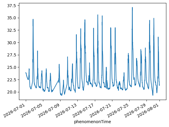

# Analysis of days above 35 degress per month

dfHot = df[df["Temp"] > 35.0].copy()

# Group by month and count unique days
daysCount = dfHot.groupby(dfHot.index.to_period("M")).apply(
    lambda g: len(set(g.index.date))
)

daysCount

C:\Users\saulm\AppData\Local\Temp\ipykernel_13140\3681847772.py:6: UserWarning: Converting to PeriodArray/Index representation will drop timezone information.
  daysCount = dfHot.groupby(dfHot.index.to_period("M")).apply(





phenomenonTime
2026-04    1
2026-05    3
2026-06    4
2026-07    3
2026-08    2
2026-09    2
Freq: M, dtype: int64

# Plot using index directly
plt.figure(figsize=(8, 4))
sns.barplot(x=daysCount.index.astype(str), y=daysCount.values, color="crimson")
plt.title("Days over Temp > 35°C")
plt.xlabel("Month")
plt.ylabel("Days")
plt.show()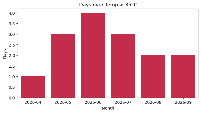

# 1. Filter readings > 30°C
hot_df = df[df["Temp"] > 30]

# 2. Count 15-min intervals per day and filter days with >= 8 intervals (2 hours)
daily_counts = hot_df.groupby(hot_df.index.date).size()
validDays = pd.to_datetime(daily_counts[daily_counts >= 8].index)
validDays[:5]

DatetimeIndex(['2026-03-26', '2026-04-11', '2026-04-14', '2026-04-15',
               '2026-04-16'],
              dtype='datetime64[ns]', freq=None)

# 2. Group by month and count
monthlyCounts = validDays.to_series().groupby(validDays.to_period("M")).count()

monthlyCounts

2026-03    1
2026-04    7
2026-05    4
2026-06    1
2026-07    5
2026-08    4
2026-09    6
Freq: M, dtype: int64

# Plotting with Seaborn
plt.figure(figsize=(8, 4))
sns.barplot(
    x=monthlyCounts.index.astype(str),
    y=monthlyCounts.values,
    color="darkorange",
)

plt.title("Days with 2 Hours Above 30°C")
plt.xlabel("Month")
plt.ylabel("Number of Days")
plt.tight_layout()
plt.show()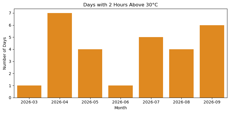

# 1. Calculate 2-hour temperature difference (8 intervals of 15 min)
# diff(8) calculates: temp[t] - temp[t - 2 hours]
temp_diff_2h = df["Temp"].diff(8)

# 2. Filter timestamps where temperature dropped more than 5°C
drops = df[temp_diff_2h < -5]

# 3. Get unique dates with drops and group by month
dropDates = pd.DatetimeIndex(pd.Series(drops.index.date).unique())
dropDates[:5]

DatetimeIndex(['2026-03-27', '2026-03-29', '2026-03-30', '2026-03-31',
               '2026-04-01'],
              dtype='datetime64[ns]', freq=None)

monthlyDropDays = (dropDates.to_series().groupby(dropDates.to_period("M")).count())
monthlyDropDays

2026-03     4
2026-04     9
2026-05     5
2026-06    11
2026-07     9
2026-08     8
2026-09     8
Freq: M, dtype: int64

# 4. Plot using Seaborn
plt.figure(figsize=(8, 4))
sns.barplot(
    x=monthlyDropDays.index.astype(str),
    y=monthlyDropDays.values,
    color="steelblue",
)

# Customize chart
plt.title("Days per Month with a >5°C Temperature Drop in 2 Hours")
plt.xlabel("Month")
plt.ylabel("Number of Days")
plt.tight_layout()
plt.show()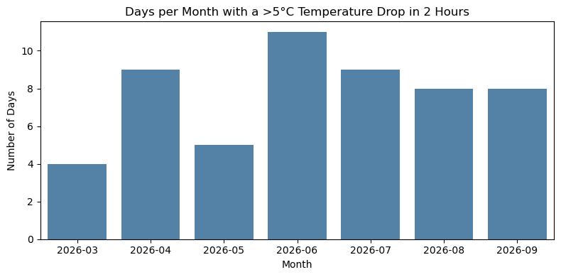

Input data

You can download the input data from this link.