Groundwater modeling figures and related topics
/Groundwater modeling figures and related topics
Read MoreGroundwater modeling figures and related topics
Read MoreBasic example of MODFLOW 6 groundwater flow modeling with Flopy. The model is multilayered and runs on transient conditions with the recharge, well and river boundary conditions implemented. The example also load model results and create head distributions with flow direction plots with Matplotlib.
The example runs entirely on the Google Colab platform with the use of a Github repository with the MODFLOW 6 executables. This workflow is intended to give a complete online experience of groundwater modeling without any particular computer/software requirement.
Read MoreGroundwater modeling with several boundary conditions and complex hydrogeological setups require advanced tools for mesh discretizacion that ensures adequate refinement in the zone of interest while preserving a minimal cell account. Type of mesh has to be engineered in a way to preserve computational resources and represent adequately the groundwater flow regime.
Read MoreWe have developed an applied case of groundwater model discretized from ESRI Shapefiles with refinement areas. Boundary conditions are also set up from spatial data with the intersect functionality of Flopy. Model surface and layer bottom are imported / processed from xyz point data. The simulation is run for one steady and ten transient stress periods and results are plotted for head on aerial view and cross section.
Read MoreIn order to improve the accuracy of a groundwater flow simulation we need a strong conceptual model, a high quality observation dataset and a numerical code that can handle specific characteristics of the groundwater flow we want to evaluate. MODFLOW 6 can deal with variable density flow with the BUY package and also with variable viscosity with the VSC package that is implemented on the latest versions of Model Muse. This tutorial covers an applied case of variable viscosity modeling due to the injection of salinity and heat to a model with regional groundwater flow. The main features for the implementation of the VSC package are explained and the resulting concentrations on two observation points are evaluated with Flopy codes.
Read MoreWith Model Muse and MODFLOW6 DISV you can model faults and fractures having small cells close to the fracture alignment. In order to achieve small cell sizes close to the fracture aligment the normal MODFLO6 discretization schema (columns and rows) creates a series of unused/unwanted cells, but MODFLOW6 came with two new discretization options that allow us to have local refinements close to areas of interest decreasing the total amount of cells and thus the decreasing computational time.
Read MoreSpatial discretization for a mine related groundwater model has to come from geospatial data that has a system of reference (crs). The latest version of Modflow that is Modflow 6 implements the discretized by vertices option (DISV) that allows the creation of triangular, quadtree, voronoi meshes among other options. We have developed some Python scripts to create voronoi meshes from shapefiles where the user has to define a limit polygon, layers (point, line or polygon) and refinement levels. The code generates meshes with adequate performance and gives geospatial output for the final voronoi mesh as well as the intermediate steps.
Read MoreGroundwater model creation requires a complete set of spatial data for the different hydraulic parameters, boundary conditions and other model items. Vector and raster data need to be preprocessed, converted, reprojected to fit the requirements of Model Muse.
This tutorial covers an applied case of raster and vector data processing for a basin.
Read MoreOne of the greatest new features of the latest Model Muse version is the implementation of the BUY package for variable density and seawater intrusion modeling. The BUY package was already available in Modflow 6 but the resources to build a model was limited to scripts in Flopy or to build the packages for Modflow by hand, now with Model Muse much stress and pain could be relieved to simulate this type of groundwater model much relevant on the current climate change scenarios.
This tutorial shows the complete procedure to implement variable density / seawater intrusion modeling on a simple coastal aquifer with regional flow. The model runs over two steady / transient stress periods of 50 year each and has a cell with of 20 on the intrusion and 15 layers.
Read MoreEven though that the version 5.2 was released on March 22 2024 we just found time to make a video explaning the new features of this version and where they are implemented on the graphical user interfase. This new version of Model Muse allows to simulate variable density and variable viscosity flow among other features of Modflow 6. Have a look on the video and wait for our comming applied tutorials related to these new features.
Read MoreGenerating 3D visualizations of groundwater models is essential to analyze the flow regime, perform quality checks and see the interaction of the groundwater body with external factors / boundary conditions. The Flopy library has tools to export the parameters, boundary conditions and results that we have modified and compiled within a Python class. The use of this class allows the generation of Vtk files on a friendly way and in few steps. The tutorial also includes a representation of the parameters generated in ParaView.
Read MorePython has awesome packages for machine learning that can be coupled to groundwater models and perform automatic calibration of hydraulic parameters. This tutorial covers the procedure to implement a neural network based on a set of parameters set with corresponding head values; the study case is on a transient pumping test model with an observation point located around 10 meters away from the pump well. The analysis predicts the calibration parameters from the spatially interpolated observed head values.
Read MoreWe did this tutorial since the documentation or examples on the topic were not available. Flopy can export the model grid and model attributes to shapefile with a coordinate system of reference for the three types of discretizations of MODFLOW 6. We have done an applied example to export the grid of a discretized by vertices model (DISV) to the ESRI Shapefile model. The tutorial also show options for the final grid representation in geopandas.
Read MoreThis tutorial covers the whole procedure to perform a sensitivity analysis over a 72 hour pumping test plus recovery on the hydraulic response in an observation piezometer located at 11 meters from the well. the Since the study case it’s a transient model the sensitivities will vary over time and stage of pumping/recovery.
Read MoreHaving a geological model can enhance numerical models since it allows to represent higher accuracy the potential distribution of hydraulic parameters in the horizontal and vertical direction. The process to implement/insert a geological model into a Modflow model is a challenge due to restrictions on proprietary software and spatial tools; we have done the whole procedure to insert a geological model into a MODFLOW-NWT groundwater model with scripts in Python, Pyvista and others.
The code extracts the cell centroids of the modflow model and then compares its position with the different geological units exported from Leapfrog to Vtk. Once the corresponding lithology of the cell is identified a hydraulic parameter is assigned. The tutorial works from Vtks of a geological model done in Leapfrog, but it can work with any Vtk.
Read MoreThis tutorial shows the complete procedure to convert a geological unit as a Leapfrog mesh (*.msh) to the VTK (Visualization Toolkit) format using Python and GemGIS. Follow these steps to seamlessly transfer your geological data for advanced visualization, analysis and comparison with other model results.
Read MoreBased on a coupled workflow on QGIS and Python it is possible to extract the required information for a Gempy model and run it for defined voxel sizes. This tutorial covers the whole procedure of spatial data preparation, data preprocessing in defined formats and geological modeling with Python and Gempy.
Read MoreWe have done an applied groundwater model for a pumping test on a confined aquifer. The wellsite is located on the Clairborne aquifer (Georgia, USA) and has two observations on different layers besides the well itself. The aquifer test has two periods of pumping and recovery that last 3 days each one and the numerical model was constructed with MODFLOW-6 based on a Python script with the FloPy package. Comparison among observed and simulated wells were done with plots in Matplotlib.
Read MoreGenerating 3D visualizations of groundwater models is essential to analyze the flow regime, perform quality checks and see the interaction of the groundwater body with external factors / boundary conditions. The Flopy library has tools to export the parameters, boundary conditions and results that we have modified and compiled within a Python class. The use of this class allows the generation of Vtk files on a friendly way and in few steps. The tutorial also includes a representation of the parameters generated in ParaView.
Read MoreModflow on parallel processing seemed to lie in the far-off future, but now it’s possible to take advantage of most of your cores to run parallelized versions of MODFLOW 6. Since most MODFLOW modelers work on Windows we wanted to bring something more than a “packed” solution; our goal was to bring an enriched “packed” experience.
Read More
ONLINE COURSES:
LATEST POSTS
SEARCH


 |
 |
 |
 |
 |
 |