Basic HEC-RAS tutorial
/HEC-RAS 5.0 now has a user interface that includes the RAS Mapper, which is used for 2D modeling. It is also possible to see the results in an interactive way.
Here we will present the steps and needed considerations to model river/channel flow in HEC-RAS. This example consists on a water channel that overflows. Referential parameters will be used.
Steps
Once HEC/RAS 5.0 is installed, change the system units in Options > Unit System (US customary SI). The next window will be seen. Here, we will change the system units to System International and set it as default for new projects.
To generate a new project:
File > New Project
You will see this window where you will assign a name to the project.
After creating the project file, we need to create the Geometry Data File.
Edit > Geometric Data
And you will see the Geometric Data editor which has a menu with options to create a river network, like junctions, cross sections, bridges, structures, storage areas and pump stations.
We will create a river network with the River Reach tool. Draw the river and once it is finished, double click. A new window will appear where you need to give a name to the River and the Reach. Finally click OK.
Now, we need to create the cross sections. Click on the Cross Section icon. Here we will insert information about the sections like coordinates, reach lengths, Manning coefficient, channel overbanks and contraction/expansion coefficients.
To add a new cross section, go to Options > Add a new cross section.
When adding a new Cross Section, we need to assign a number. In this case the number is the highest because it corresponds to the upstream section. After this, click OK.
Insert the information for each section. In this case we are working with a simple cross section. Click Apply Data to show the geometry.
To create new cross sections, in this case, we will copy the initial one with Options > Copy current Cross section
Proceed to save the Geometry Data File with File > Save Geometry Data.
After creating the geometry files, we are going to create the ones corresponding to Permanent Flow.
Go to Edit>> Steady Flow Data.
Here we can add several profiles. In this opportunity we will create two, which correspond to the two flows we want to simulate.
To add the boundary conditions data, click Reach Boundary Conditions and we can choose from four different boundaries: Known W.S, Critical Depth, Normal Depth and Rating Curve.
In this case we will choose Normal Depth for the downstream boundary condition. The next image shows the window where we need to enter, in this case, the downstream slope.
After saving the Flow Data, we can start the simulation.
Run > Steady Flow Analysis
In the following window we can create different scenarios combining flow data files with geometry data files. After specifying the Flow Regime, click Compute to start the simulation.
To see the results, click:
- View cross section: To see the cross section, water level, energy line.
- View profiles: To see the longitudinal profile results with the water level and energy line.
- View summary output tables by profile: To see the tabular results including velocity, energy slope, Froude number, among others.


