Modflow 6 has a new approach in setting up observation points and it's essentially different to the previous versions. The OBS6 package works not only with heads and drawdowns but also with flows, so it's also possible to calibrate the model against baseflow or any other recorded flow from a boundary condition directly. We have created an applied case of the implementation of piezometers in a hillslope groundwater flow model in Modflow 6 and Model Muse. The tutorial covers all the steps related to the implementation of the observed points in Model Muse as well as the comparison among simulated and observed heads through scripts in Flopy.

Tutorial

Code

This is the code for simulated vs observed heads representation:

#import the require packages
import flopy
import pandas as pd
import numpy as np
import matplotlib.pyplot as plt

#define model name and model path
modelWs = '../Model/'
modelName = 'HillslopeModel_v1'
namFile = modelName+'.nam'

#open the observation file out heads
obsOut = flopy.utils.observationfile.Mf6Obs(modelWs+modelName+'.ob_gw_out_head.csv',isBinary=False)

#create a dataframe for the observation points
totalObsDf = obsOut.get_dataframe().transpose()
totalObsDf = totalObsDf.rename(columns={totalObsDf.keys()[0]:'SimHead'})
totalObsDf = totalObsDf.drop('totim',axis=0)
totalObsDf['ObsHead'] = 0
totalObsDf['Lat'] = 0
totalObsDf['Lon'] = 0
totalObsDf.head()

	SimHead	ObsHead	Lat	Lon
HD_OBS_474820122185601	1.045374e+02	0	0	0
HD_OBS_474851122165301	1.084544e+02	0	0	0
HD_OBS_474907122194901	-1.000000e+30	0	0	0
HD_OBS_474909122164401	1.096796e+02	0	0	0
HD_OBS_474923122195601	-1.000000e+30	0	0	0

#open the observed data file
obsDf = pd.read_csv('../Txt/HobDf.csv',index_col=0)
obsDf.head()

	SiteNo	Latitude	Longitude	LatLonDatum	SurfaceElevation_m	SiteCode	ScreenElevation_m	WTElevation_m
0	12126800	47.825556	-122.254167	NAD83	96.6216	Obs_12126800	NaN	NaN
1	12128100	47.884461	-122.299211	NAD83	124.9680	Obs_12128100	NaN	NaN
2	12128130	47.909753	-122.297894	NAD83	97.5360	Obs_12128130	NaN	NaN
3	474758122192101	47.822041	-122.298186	NAD83	119.9810	Obs_474758122192101	78.2234	NaN
4	474820122185601	47.814541	-122.306520	NAD83	107.7890	Obs_474820122185601	39.2090	88.1294

#look for the observed elevation and coordinates
for index, row in totalObsDf.iterrows():
    for index2, row2 in obsDf.iterrows():
        if index[7:] == str(row2.SiteNo):
            totalObsDf.loc[index,'ObsHead'] = row2.WTElevation_m
            totalObsDf.loc[index,'Lat'] = row2.Latitude
            totalObsDf.loc[index,'Lon'] = row2.Longitude

#compute the residual and save csv file
totalObsDf = totalObsDf[totalObsDf['SimHead']>0]
totalObsDf['Residual'] = totalObsDf['SimHead'] - totalObsDf['ObsHead']
totalObsDf.to_csv('../Txt/HobDf_Out.csv')
totalObsDf.head()

	SimHead	ObsHead	Lat	Lon	Residual
HD_OBS_474820122185601	104.537359	88.129400	47.814541	-122.306520	16.407959
HD_OBS_474851122165301	108.454441	115.713800	47.813986	-122.282630	-7.259359
HD_OBS_474909122164401	109.679565	113.885000	47.818986	-122.280130	-4.205435
HD_OBS_474953122170201	108.180467	123.665778	47.830930	-122.286520	-15.485311
HD_OBS_475044122155601	108.793058	80.357000	47.845374	-122.266797	28.436058

totalObsDf

	SimHead	ObsHead	Lat	Lon	Residual
HD_OBS_474820122185601	104.537359	88.129400	47.814541	-122.306520	16.407959
HD_OBS_474851122165301	108.454441	115.713800	47.813986	-122.282630	-7.259359
HD_OBS_474909122164401	109.679565	113.885000	47.818986	-122.280130	-4.205435
HD_OBS_474953122170201	108.180467	123.665778	47.830930	-122.286520	-15.485311
HD_OBS_475044122155601	108.793058	80.357000	47.845374	-122.266797	28.436058
HD_OBS_475104122191901	55.070670	69.384200	47.850930	-122.323189	-14.313530
HD_OBS_475106122170101	104.033737	114.494600	47.851485	-122.284854	-10.460863
HD_OBS_475120122162401	108.820731	123.029000	47.855374	-122.274576	-14.208269
HD_OBS_475150122192101	40.718962	41.590660	47.863707	-122.323745	-0.871699
HD_OBS_475328122181901	65.566638	43.476200	47.890929	-122.306523	22.090438
HD_OBS_475334122180401	72.714256	72.279800	47.892596	-122.302357	0.434456

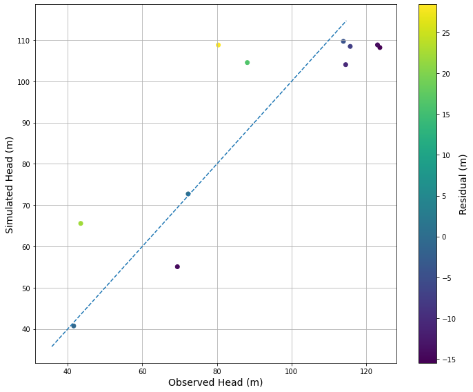
#Create a basic scatter plot with Matplotlib
#A identity line was created based on the minumum and maximum observed value
#Points markers are colored by the residual and a residual colorbar is added to the figure
fig = plt.figure(figsize=(10,8))
x = np.linspace(totalObsDf['SimHead'].min()-5, totalObsDf['SimHead'].max()+5, 100)
plt.plot(x, x, linestyle='dashed')
plt.scatter(totalObsDf['ObsHead'],totalObsDf['SimHead'], marker='o', c=totalObsDf['Residual'])

cbar = plt.colorbar()
cbar.set_label('Residual (m)', fontsize=14)

plt.grid()
plt.xlabel('Observed Head (m)', fontsize=14)
plt.ylabel('Simulated Head (m)', fontsize=14)
fig.tight_layout()