How to calculate a Terrain Volume with QGIS3 - Tutorial

Calculate volumes is an easy task on QGIS 3 with the use of SAGA GIS tools under the Processing toolbox. Raster volumes can be calculated above or below a base level and two other specific calculation, input rasters need to be in UTM. These type of calculation is useful for earth movement, reservoir design, risk analysis and other spatial analysis.

The tutorial presented on this post shows the complete procedure to calculate the raster volume above a base level on QGIS3.

Read More


Suscribe to our online newsletter

Subscribe for free newsletter, receive news, interesting facts and dates of our courses in water resources.


Watershed and Stream Network Delimitation with Python and Pysheds - Tutorial

What would happen if we shift our GIS geoprocessing to Python? What would happen if we treat our raster and vector spatial data as objects and variables on a Python 3 script? Then we can ask ourselves if it is neccessary to reinvent the wheel, it is necessary to change a workflow that already work on a GIS software.

There is a simple answer to this dilemma: More control

Working with Python give us more control on the geoprocessing itself since we leave the Graphical User Interface (GUI) with its icons, buttons and dialog boxes. With Python running on a Jupyter Notebook, we can link with specific files, define geoprocess and it options, make plots of draft and final data, and export results to vector/raster SIG formats. There are other advantages of spatial analysis in Python which are the reproducibility and the processing speed.

Read More


Suscribe to our online newsletter

Subscribe for free newsletter, receive news, interesting facts and dates of our courses in water resources.


Available QGIS tools and plugins for hydrological modeling - Review

QGIS is viewed as a software for the spatial data processing to create the input data for a hydrogeological modeling as HEC-HMS or RS-Minerve. But, are there any hydrological software that can run on the QGIS interface? There are some half answers and complete answers that we will answer in this article.

Read More


Suscribe to our online newsletter

Subscribe for free newsletter, receive news, interesting facts and dates of our courses in water resources.


Spatial Manipulation of a Autocad DXF File with Python3 and GeoPandas - Tutorial

In GIS the objects are related to a spatial location. Usually there is no need to modify a location since spatial data comes from field work or other surveys. When we work with CAD files as DXF (Autocad Drawing Exchange Format) files, sometimes the spatial data is available as a layout view and not as a model view. The layout data is on local coordinates, and at specific scale therefore we need to scale and translate the spatial data to “return” it to its original spatial location and extension.

We tried to make this job with Inkscape and QGIS3, but we were unsuccessful to complete the scale and translation. While working with the DXF in Inkscape, each object selection, layer order combination, object ungrouping took several minutes and the results were poor. At the lowest motivational stage of this spatial request, we thought that it might me something in Python that can be useful for this.

On a internet search, we found that the spatial version of the Pandas data analysis library: Geopandas was capable not only to open the DXF files, but also to scale, translate, and filter spatial data according to specific criteria. Geopandas is capable to export spatial data in different formats and to plot data interactively on a Jupyter Notebook.

This tutorial shows the procedure to open a DXF file in Python pandas, perform scale and translation to place the spatial features on their original position, filter unwated objects on the layout view and export results to QGIS3 as shapefile.

Read More


Suscribe to our online newsletter

Subscribe for free newsletter, receive news, interesting facts and dates of our courses in water resources.


Groundwater Quality Analysis with QGIS3 Tutorial - Case Arsenic in California

Physical process on the surface and underground flow regime are spatially and temporal distributed, therefore the use of GIS software is key to understand the different patterns in groundwater flow and quality and the interaction with surface flow, geology and anthropogenic factors.

QGIS is a open geographical information system (GIS) software that brings a variety of tools for the thematic spatial representation of the groundwater quality components. This tutorial shows a whole exercise of data preparation, color based representation, ruled based representation of points above standars, spatial interpolation and contour representation.

Read More


Suscribe to our online newsletter

Subscribe for free newsletter, receive news, interesting facts and dates of our courses in water resources.


How to smart download OpenStreetMap spatial data with QGIS3 and QuickOSM

OpenStreeMap (OSM) is a collaborative project to create a world spatial database. This project is motivated by the availability of map information around the world. The database is on continuous growth, it has more than 6.3 thousand million GPS points, around 5 million users and 1 million contributors.

The procedure to download spatial data from OSM has changed from previous QGIS version. Now in QGIS3 there are multiple options to download data from OSM; this tutorial show the installation, and operation of the QuickOSM plugin to perform smart access to the OSM database in QGIS.

QuickOSM works with the Overpass API that was developed to serve up custom selected parts of the OSM map data. This API is optimized for data consumers and it can allow the access millions of elements in some minutes with a specified search criteria (location, object type, tags, proximity or combinations of them).

Read More


Suscribe to our online newsletter

Subscribe for free newsletter, receive news, interesting facts and dates of our courses in water resources.


Overview of QuickMapServices Plugin for Basemaps in QGIS3 - Tutorial

QGIS 3 has a lot of new features and new tools for geoprocessing and spatial analysis, however there are some tools from QGIS 2 that hasn´t migrated yet. An example of this break was the OpenLayers plugin, one of the most popular and first plugins in QGIS 2 that is not available in the new version of QGIS.

OpenLayers plugin provide maps from Google, OSM and Bing in QGIS 2. Basemaps in QGIS 3 can be inserted as a XYZ Tiles on a process described on this tutorial. However, QuickMapServices plugin allow the search and implementation from a set of basemaps on different formats (TMS, WMS, WFS and GeoJSON) in QGIS 3.

Read More


Suscribe to our online newsletter

Subscribe for free newsletter, receive news, interesting facts and dates of our courses in water resources.


Basic Example of QGIS - HECRAS Geometry Construction and Flood Simulation

Flow simulation is an important task for engineering and disaster management. From the free softwares available for flow simulation, HEC-RAS is a strong alternative for its continuous development, the capability to simulate many flow types, and the interaction with other softwares like QGIS or MODFLOW.

QGIS is a free and open source software Geographical Information System (GIS) application. There is a environment of available plugins in QGIS that perform specific tasks of analysis, representation and preprocessing. There are QGIS plugins related to HEC-RAS, in this tutorial we will use the Q-RAS plugin to develop a basic example of flow model geometry construction in QGIS and steady flow simulation in HEC-RAS.

Read More


Suscribe to our online newsletter

Subscribe for free newsletter, receive news, interesting facts and dates of our courses in water resources.


Flood Monitoring Tutorial with Sentinel 2 and Landsat 8 Images in QGIS 3

With current technology and the availability of remote sensing tools through different servers makes it possible to determine or estimate the areas that are flooded or could be, the focus of this tutorial in which a methodology to determine flood zones will be described from the calculation of the NDVI and compare the results with the use of two servers, Sentinel 2 and Landsat 8.

Read More


Suscribe to our online newsletter

Subscribe for free newsletter, receive news, interesting facts and dates of our courses in water resources.


Vegetation and Biomass Indices Estimation with QGIS 3 - Tutorial

The vegetation indices are obtained from area and satellite images and can be used to estimate changes in the state of vegetation, biomass, leaf area index and chlorophyll concentration. The determination of vegetation indices is calculated from the relationship between the reflectance of the electromagnetic spectrum. While biomass presents various methodologies to be able to estimate that they are based on field measurements that despite being a direct method are still very limited. Currently, the use of remote sensors provides a method to generate information on biomass.

In this tutorial the estimation and relationship of the biomass of a study area with the Normalized Difference Vegetation Index (NDVI) and the Normalized Red-Green Difference Index (NGRDI) will be carried out.

Read More


Suscribe to our online newsletter

Subscribe for free newsletter, receive news, interesting facts and dates of our courses in water resources.


Determination of mine polluted lakes with QGIS 3 and SCP 6 - Tutorial

Mining and the treatment of metals are a significant source for the contribution of pollutants in various natural resources such as lakes. The impact of a pollutant on the lakes depends on the physical and chemical conditions that affect its toxicity and the degree of exposure related to concentration and time. The contribution of metals can be incorporated by precipitation, mine filtration, soil washing, leaching and percolation.

Read More


Suscribe to our online newsletter

Subscribe for free newsletter, receive news, interesting facts and dates of our courses in water resources.


Spectral signature behavior analysis for seawater quality with QGIS 3 and SCP plugin - Tutorial

Remote sensing allows the interpretation of dynamic processes in a study area at a spatial and temporal level. This information is collected from the surface that is captured by a sensor located on board a satellite in orbit around the earth. In this way, you can compare images and analyze the changes of a study area.

Different space agencies have facilitated access to information provided by satellites through servers and web portals, where satellite images can be downloaded for the analysis and interpretation of resources, for this instance, the quality of seawater can be analyzed through the classification of specific footprints using geographic information systems tools such as QGIS 3 and the Semi-Automatic Classification plugin.

Read More


Suscribe to our online newsletter

Subscribe for free newsletter, receive news, interesting facts and dates of our courses in water resources.


Extracting geological faults and orientation representation in QGIS with GeoTrace - Tutorial

Image from earth surface are available from satellite images and unmanned aerial vehicules (UAV). Image resolution ranges from 10 meters on free available datasets as Sentinel2, less than 1 meter on commercial satellite imagery to 0.05m (or even less) from UAVs.

Scikit-image is a library for image processing in Python. Currently there are few QGIS plugins that run Scikit-image, we found one that extracts geological features as fractures and represent fault dip, dip direction, and strike in stereonets and rose diagrams. This tutorial show the procedure to install GeoTrace on QGIS 3 with its dependencies, runs a geological fault trace on a modified raster, calculate fault strike azimuths as a separate attribute field represent them as a strike rose.

Read More


Suscribe to our online newsletter

Subscribe for free newsletter, receive news, interesting facts and dates of our courses in water resources.


How to open HDF files on Sinusoidal Coordinate System in QGIS3 with PyQGIS - Tutorial

For a normal GIS user, QGIS 3 brings a lot of new tools, new forms to perform spatial analysis but also it doesn´t bring (yet) some options available in QGIS 2. This is the case for the representation of HDF raster files that is not available in QGIS 3 but it is available in QGIS 2. Research have been performed to address this issue and many options were evaluated to open the HDF files and perform a geotransformation from Sinusoidal Coordinate System to Geographical Coordinate System.

The solution came from the powerful gdal library and some core Python functions. This tutorial show the procedure to open a layer of a MOD13A2, a MODIS data product for vegetation evaluation and reproject it to geographical coordinate system (lat/lon).

Read More


Suscribe to our online newsletter

Subscribe for free newsletter, receive news, interesting facts and dates of our courses in water resources.


Land cover spectral signatures determination with QGIS 3 and Semi-Automatic Classification Plugin (SCP 6) - Tutorial

There are several satellites with different characteristics that acquire multispectral images of the surface of the earth. In this case, the Sentinel 2 images are particularly useful for the monitoring of land cover and can be provided free of charge from SCP.

In this tutorial we will perform the evaluation of spectral signatures using the Semi-automatic Classification complement in version 6, which is a free open source plugin for QGIS 3 that allows the supervised and unsupervised classification of remote sensing images.

Read More


Suscribe to our online newsletter

Subscribe for free newsletter, receive news, interesting facts and dates of our courses in water resources.


How to visualize water quality data in QGIS 3? From points to raster to contour lines - Tutorial

Spatial interpolation techniques used to evaluate estimations of physical and chemical constituents in areas where they are not estimated (Murphy et al., 2009). This tutorial will show how to interpolate data from point data to obtain a raster that covers the study area and, then, to obtain contour lines from the raster.

The Inverse Distance Weighted (IDW) method is one of the most used due to its simplicity. IDW expect that each point has a nearby impact that reduces with distance. It gives more weight to the points nearest to the forecast area. QGIS has the ability to perform this interpolation method by using data points and the result is displayed as a raster file.


Read More


Suscribe to our online newsletter

Subscribe for free newsletter, receive news, interesting facts and dates of our courses in water resources.


How to calculate the Root Mean Square Error (RMSE) of an interpolated pH raster?

The root mean square error (RMSE) has been used as a standard statistical parameter to measure model performance in several natural sciences. The parameter indicates the standard deviation of the residuals or how far the points are from the regression or modelled line. The following figure shows the residuals as green arrows and its location between the point data and the regression line. 

Read More


Suscribe to our online newsletter

Subscribe for free newsletter, receive news, interesting facts and dates of our courses in water resources.


Electric Conductivity Analysis of a River Pathway using QGIS 3 and the Profile Tool Plugin

Electrical Conductivity (EC) has been used to analyze the content of dissolved salts in water. EC refers to the ability to transmit electricity (Ikeda et al. 1991). Pure water has low values of EC because the electricity is conducted by the ions in solution; therefore, the greater the concentration of ions in water, the greater the value of EC. This tutorial explains how to analyze the EC of a river using the Profile Tool plugin in QGIS 3.0.

Read More


Suscribe to our online newsletter

Subscribe for free newsletter, receive news, interesting facts and dates of our courses in water resources.


How to visualize time series in QGIS 3.0 with the Time Manager Plugin - Tutorial

Time series in hydrology can be analyzed to a) detect a trend due to another random hydrologic variable, b) develop and calibrate a model, c) predict future characteristics of a variable (Machiwal & Jha 2012). The application of time series analysis is diverse; for instance, it can be used to evaluate global trends of soil moisture (Dorigo et al. 2012), to analyze river discharges (Papa et al. 2012), to detect glacial lake outburst floods (Veh et al. 2018) or to detect rainfall patterns (Wang et al. 2016).

The visualization of the data variability over the time can be a useful tool to identify patterns or to compare the behavior of different samples. The use of software for Geographic Information Systems (GIS) allows to identify the location of the samples and to compile the information that the samples have. Open-source software like QGIS offers excellent tools to achieve this objective. This tutorial will explain how to use the Time Manager Plugin.

Read More


Suscribe to our online newsletter

Subscribe for free newsletter, receive news, interesting facts and dates of our courses in water resources.


Comparison of IMERG Precipitation with Station Information with QGIS, Python and Pandas - Tutorial

There are tools for temporal data analysis like Python, IPython and Jupyter; there are tools for spatial data analysis like QGIS. But, are there tools for spatio-temporal analysis? Unfortunately no, but there are good approaches to manage spatial data in Jupyter or to run IPython in QGIS3. These approaches aren't a complete ansqwe to the current demands of big data processing in few computational time with simple scripts, but by sure it will help to shape better solutions.

Read More


Suscribe to our online newsletter

Subscribe for free newsletter, receive news, interesting facts and dates of our courses in water resources.