How to decrease the Raster Resolution in QGIS3 - Tutorial

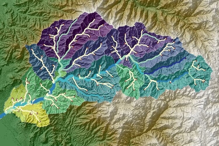
A raster is a rectangular pattern of rows and columns with a spatial georeferentiation. On a raster each cell contains a value that is uniform in the cell geospatial extension and its the most used spatial data model when we deal and analyze spatially distributed values as land cover, precipitation or population density.

Spatial analysis on raster deals with raster resolution or cell size. As smaller the cell size, the result from the analysis will be finer however the raster file size will be much larger; if we use coarse cells, the raster file sizes will be smaller but the results could be poor for the objectives of the analysis. An equilibrium in between the raster resolution and the raster file size has become a topic to have in mind for beginner GIS users as well as for experienced GIS users.

QGIS is a free and powerful Geographical Information Software (GIS) software. QGIS comes with a variety of tools to manage vector and raster spatial data and its capabilities can be increased when it couples with Grass, SAGA GIS, OTB and its plugins. This tutorial show the simple procedure to change the raster resolution in QGIS 3.

Read More


Suscribe to our online newsletter

Subscribe for free newsletter, receive news, interesting facts and dates of our courses in water resources.


How to insert Recharge Data Values correlated with Elevation into Model Muse - Tutorial

One of the main boundary conditions of the groundwater flow systems is the recharge. This is a process where water from the surface moves downward reaching the groundwater. The rate of recharge can be influenced by several factors like water content of surface materials, type of soil, plant cover and precipitation rate.

Model Muse is a versatile MODFLOW graphical user interface (GUI) where it is possible to insert many boundary conditions and terrain characteristics in order to represent the real conditions of the groundwater flow in an accurate way.

In this tutorial, we are considering a case study where the recharge rate is correlated with the elevation which is a characteristic of Andean basins. We will show you how to insert this correlation of recharge-elevation values into Model Muse in order to have a better representation of the hydrological cycle of this basin.

Read More


Suscribe to our online newsletter

Subscribe for free newsletter, receive news, interesting facts and dates of our courses in water resources.


Key Concepts for Groundwater Management in Arid Regions

If we compare the amount of hydrologist vs. the amount of hydrogeologist, we can see that there is a gap in between the number of specialists in surface water and groundwater. Traditionally, the hydrology as a academic course is related to surface hydrology while the underground hydrology (hydrogeology) has been scarcely treated in typical undergraduate or graduate studies. As a comparison with then chicken and the egg, the lower or less popular academic opportunities in hydrogeology has produced a limited number of groundwater specialist who deal with a limited sort of groundwater studies.

Read More


Suscribe to our online newsletter

Subscribe for free newsletter, receive news, interesting facts and dates of our courses in water resources.


Geospatial Referentiation of a MODFLOW Model with Flopy - Tutorial

Groundwater models are geospatial referenced (unless you are in a laboratory) since we represent the actual and future conditions of a certain porous / fractured media, however the actual model matrix resolution is spatially independent since it deals with a hydrogeological conceptualized array of columns, rows and layers. The nexus in between the matrix and the groundwater flow system has been a topic in the model development, even later versions of Model Muse ask for the model system of reference (as EPSG or Proj4 code), however the user has to keep in mind the water heads and where those water heads are located.  The USGS has developed a Python package called Flopy for the model construction, simulation and output representation; this package has interesting features for the interaction with the input and output data and for the georeferentiation of model data. This tutorial shows the complete procedure to geospatial reference a MODFLOW NWT model with some lines of Python code in a Jupyter Notebook and the representation of geospatial referenced model discretization data in QGIS 3.

Read More
 

Suscribe to our online newsletter

Subscribe for free newsletter, receive news, interesting facts and dates of our courses in water resources.


Exploring the QGIS 3 options to create maps - Tutorial

Map creation is one of the most or maybe the most popular application of Geographical Information System (GIS) software as QGIS. There has been an evolution in the layout options along the previous versions and now QGIS 3 has a whole set of map elements as legends, attribute tables, arrows, lines, scales among others. Each map element has a entire set of tools to be customized to the canvas spatial reference or other spatial data properties and styled to the desired output. Map design quality is upon the user and his experience and knowledge of the available tools in QGIS 3. This tutorial shows the procedure to create a layout / map, reviews the map objects, implements some objects in a applied case and export the map as pdf. 

Read More


Suscribe to our online newsletter

Subscribe for free newsletter, receive news, interesting facts and dates of our courses in water resources.


How to add a Google Map/Terrain/Satellite Layer in QGIS 3 - Tutorial

QGIS is a open source and powerful Geographic Information System (GIS) software. The latest version of QGIS is QGIS 3.0 that comes with many and exciting new features for the old and new users. As the previous versions of QGIS, the software is really intended to make more spatiall analysis and management with less effort, however this version has new tricks and a new order to locate tools. In this tutorial we will show the complete procedure to import a Google Map layer to the QGIS 3 canvas as XYZ tiles.

Read More


Suscribe to our online newsletter

Subscribe for free newsletter, receive news, interesting facts and dates of our courses in water resources.


Weather Station Tutorial Part 1: Measuring Air Temperature and Humidity in Arduino with Sensor HDC100x

Developing a low cost weather station is an interesting topic. In fact, cost of an assembled weather station is quite expensive, which can be up to €5000. Thanks for the development of an open – source electronic prototype platform Arduino, the sensor system gets into a new generation! A small-scale prototype including six sensors can be created with just only around €200 more or less. Furthermore, the creation of radio module Xbee allows the data transfer through Bluetooth channel, which makes the process of data collecting became easier and more convenient. 

Read More


Suscribe to our online newsletter

Subscribe for free newsletter, receive news, interesting facts and dates of our courses in water resources.


Basic Example of a MODFLOW Model Review, Simulation and Output Representation with Flopy - Tutorial

Flopy is a package of tools written in Python for MODFLOW groundwater flow model construction, simulation and output analysis. Flopy is build on top of well know and powerful Python packages as Numpy and works with Matplotlib and Pandas that allows to do a great amount of analysis with few lines of code. Several new capabilities in the water balance analysis can be done with Flopy bringing a better control to the modeler in terms of a more available and user friendly information of the inputs, outputs and discrepancies of the model. This tutorial shows the complete procedure to read, simulate and output analysis of a MODFLOW NWT model of a tunnel development with time. The tutorial include a discussion and review of the different tools available in Flopy and the interaction with QGIS.

Read More


Suscribe to our online newsletter

Subscribe for free newsletter, receive news, interesting facts and dates of our courses in water resources.


Introduction to Spatial Analysis in Python with GeoPandas - Tutorial

GeoPandas is the geospatial implementation of the big data oriented Python package called Pandas. GeoPandas enables the use of the Pandas datatypes for spatial operations on geometric types. The library is a combination of a set of geospatial packages in Python as Shapely, Fiona together with well known and powerful Python libraries as Numpy and Matplotlib.

For normal Geographical Information System (GIS) users, GeoPandas enables a new way to interact with geospatial data, since it allows us to handle a more variety of queries, listing, indexing and data translation in less time, and even with less computer requirements. This tutorial show some examples of data manipulation and analysis with GeoPandas for polygons and lines from Guayaquil City. 

Read More


Suscribe to our online newsletter

Subscribe for free newsletter, receive news, interesting facts and dates of our courses in water resources.


Download Climate Change Data (2006-2096) on Daily Scale from NASA NCCS Server with Python - Tutorial

There are many Global Circulation Models (GCMs) with historic and future data of Precipitation, Maximum Temperature and Minimum Temperature for different emission scenarios. Data is available on daily timescale from particular servers, in this tutorial we will show the main characteristics of the NASA NCCS THREDDS Data Server that provide the NASA Earth Exchange Global Daily Downscaled Projections (NEX-GDDP) dataset that has two of the four greenhouse gas emissions scenarios. Data from this dataset is available from 1950 to 2100 separated on historic and future with a spatial resolution of 0.25 degrees (~25km x 25 km). The tutorial show the main parts of the web server and scripts in Python to locate the closest model cell and to recursively download group of records.

Read More


Suscribe to our online newsletter

Subscribe for free newsletter, receive news, interesting facts and dates of our courses in water resources.


How to download Climate Change data from the World Bank Data API with Python

World Bank has a Climate Change Knowledge Portal with information, data and reports about climate change around the world. The portal has an Climate Data API as REST framework that can provide Precipitation and Temperature data on historic and modeled dataset from 15 global circulation models (CGMs) and 2 emissions scenarios at country and basin spatial scale. There is a Python package called wbpy that makes really easy the access to the Climate Data API by few lines of code. There are options to download data on monthly, annual and decade timescale as Python dictionary data type. This tutorial show the main parts of the API, the involved codes and a example of usage for historic and future data.

Read More


Suscribe to our online newsletter

Subscribe for free newsletter, receive news, interesting facts and dates of our courses in water resources.


Example of time-series functionality in MODFLOW 6 - Tutorial

Stress periods are defined based on particular stages on the groundwater flow conditions and requirements to hidrogeological flow regime. Time steps are mostly defined based on the computational power, desired output and convergence objectives. It can be possible that boundary conditions varies at times different from the temporal discretization defined by the stress periods and time steps. MODFLOW 6 has a time-series functionality capable of distribute the transient boundary conditions on the determined time steps. The tutorial shows a model on transient flow conditions with boundaries conditions distributed at different time intervals. A comparison of the applied well rate vs. observed pumping rate and applied constant head vs observed head has been done on a Jupyter Notebook.

Read More


Suscribe to our online newsletter

Subscribe for free newsletter, receive news, interesting facts and dates of our courses in water resources.


Example of Wetting/Drying Capabilities on Groundwater Modeling with MODFLOW 6 - Tutorial

Example of the wetting/drying capabilities in MODFLOW 6 on a groundwater model on steady and transient flow conditions. The simulation represent the groundwater flow of a 2 layer model at the following stress periods: no pumping, pumping from 2 wells, recovery from pumping in 50 days. The model has been implemented with the recharge package (RCH), river package (RIV), and well package (WEL).

The tutorial also runs some Python script for the translation of model results and boundary conditions in VTK geometry. The Python script has a interactive feature for the representation of selected stress periods and time steps. A discussion of the water table at pumping and recovery was done on the last of the tutorial.

Read More


Suscribe to our online newsletter

Subscribe for free newsletter, receive news, interesting facts and dates of our courses in water resources.


How to Calculate the Vegetation Index NDVI from Sentinel 2 Imagery with PyQGIS

Vegetation indexes are calculated from the plant radiation in certain ranges of the visible and infrared spectrum. There are many indexes based on different band combination formulas, one of the most common indexes is the Normalized Deviation Vegetation Index (NDVI) because it was of the first vegetation index and it can be applied to images from current and old satellites. This tutorial shows the complete procedure to represent in QGIS the red and near infrared (NIR) images from a clipped Sentinel 2 image with PyQGIS and then calculate the NDVI using the processing package.

Read More


Suscribe to our online newsletter

Subscribe for free newsletter, receive news, interesting facts and dates of our courses in water resources.


How to compile and run MODFLOW 6 in Mac - Tutorial

MODFLOW 6 has been compiled using gfortran on the Mac/OS operating systems. Because the program uses relatively new Fortran capabilities gfortran version 4.9 or newer must be used. If you have gfortran installed on your computer, you can tell which version it is by entering “gfortran --version” at a terminal window.

This tutorial show the procedure to compile and run MODFLOW 6 on a Terminal in MAC/OS operating sytem.

Read More


Suscribe to our online newsletter

Subscribe for free newsletter, receive news, interesting facts and dates of our courses in water resources.


Example of Transient Groundwater Flow Modeling with MODFLOW 6 - Tutorial

Based on the new file format and keywords from MODFLOW 6 it is more simple to understand a model while inspecting the input files. This tutorial show a example of a steady and transient flow model in MODFLOW 6 for a period of 30 days divided into 4 stress periods. The tutorial has a introduction to the model geometry, input files and boundary conditions, a model simulation in transient flow conditions and output visualization as VTU files in Paraview. The tutorial also includes a discussion on the water balance from the groundwater flow system at the end of the simulation.

Read More


Suscribe to our online newsletter

Subscribe for free newsletter, receive news, interesting facts and dates of our courses in water resources.


Basic Example of Groundwater Modeling in MODFLOW 6 and Visualization with Paraview and Flopy

Basic tutorial to learn the procedure to build, simulate and represent a MODFLOW 6 model. The tutorial shows a introduction to the model file system on steady state conditions. The model for this tutorial is implemented with the following boundary conditions: Drains, Recharge, Wells, and Constant Head. The grid is regular with a width of 50 meters and it has 30 rows and 24 columns; the model has 4 layers and a total thickness of 130 meters. The model is called "hatari01" and is inspired in the "twri" model from the MODFLOW 2005 documentation adapted to MODFLOW 6. The model defines a constant horizontal hydraulic conductivity as well as vertical conductivity. After the simulation a Python code is run on a Jupyter Notebook to create the Unstructured VTK files for the heads, water table and boundary conditions representation as 3D objects in Paraview.

Read More


Suscribe to our online newsletter

Subscribe for free newsletter, receive news, interesting facts and dates of our courses in water resources.


Non Overlapping Areas Determination from Multiple Layers with QGIS and PyQGIS - Tutorial

Geospatial process are involved in most part of our activities; because of that it is important to optimize the time spent by the GIS specialist and to improve the quality of the spatial analysis. PyQGIS is the Python extension in QGIS, this framework allows us to manage the QGIS tools together with Python functions and even with external Python packages improving the speed and quality of our geoprocessing and spatial representation. 

In this tutorial we will show the complete procedure to determine the non overlapping areas of an area of interest from 7 different layers.

Read More


Suscribe to our online newsletter

Subscribe for free newsletter, receive news, interesting facts and dates of our courses in water resources.


Clip Multiple Layers in QGIS with PyQGIS - Tutorial

Interesting tutorial to clip multiple polygon layers in QGIS with the Python console. The tutorial also shows a code to upload all files from a directory and store them as objects in a Python dictionary.

Read More


Suscribe to our online newsletter

Subscribe for free newsletter, receive news, interesting facts and dates of our courses in water resources.


Enhanced MODFLOW Result Representation with Python, VTK and Paraview - Tutorial

MODFLOW model output representation is key to understand the groundwater flow regime, to study the interaction with surface water and depending ecosystems and to evaluate the impact to anthropogenic and climate change requirements. Until now, there has been few open source software capable of generating3D representations and those software had limited options for color scales, cross sections and other graphical tools. On the research for more options we found Paraview, a open source software for data representation designed to analyze extremely large datasets using distributed memory computing resources.

In order to represent MODFLOW output into Paraview, a VTK file for unstructured grids is needed, this VTK type is called VTU where the "U" comes from unestructured. The tutorial show the complete procedure to process a MODFLOW model output into a VTU file and the representation in Paraview.

Read More


Suscribe to our online newsletter

Subscribe for free newsletter, receive news, interesting facts and dates of our courses in water resources.